Probabilistic Programming
Rapid model development
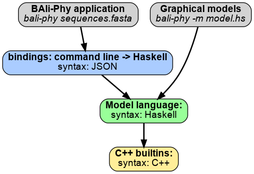
BAli-Phy 4 (unreleased) contains a language for expressing a wide range of probabilistic models. The goals of the language are:- expressivity: to be expressive enough that researchers can spend their time designing models instead of designing new inference software.
- modularity: flexibly combine smaller models to create novel larger models
- automatic inference: the inference should largely take care of itself after the model is specified.
BAli-Phy implements a universal probabilistic programming language (PPL). Universal PPLs allow inferring the number and relationship of random variables (See Ronquist et al, 2021). This differs from probabilistic graphical modeling (PGM) languages, such as Stan, BUGS, and RevBayes, where the model structure is fixed, and cannot be changed after it is initialized.
Theory: Bayesian hierarchical models as programs
A PPL allows users to write a probabilistic model in the form of a computer program. The model program draws random variables from their prior distribution, and incorporates data by calling functions to "observe" data from the data distribution. This is a natural way to write Bayesian hierarchical models.

Each time it is run, the model program will draw different values for the random variables from their prior distributions, and compute the prior probability and the likelihood of the observed data.
| run | mean | sigma | log(prior) | log(likelihood) |
|---|---|---|---|---|
| 1 | 3.000849912 | 1.130289503 | -3.24195035 | -15.5905309 |
| 2 | 5.76676590 | 0.364175082 | -2.049752039 | -1.977179616 |
| 3 | ... | ... | ... | ... |
The sequence of random choices that are made during a program run is called a trace. The trace completely determines the course of a program run, and includes all the random variables that we wish to infer. If different program runs take different branches of a conditional statement, then their traces may include different random variables. In theory a model program can be written in any language that allows (i) recording the trace for a program run, and (ii) replaying the program given a trace.
Inference under the model involves sampling from the posterior distribution of program traces. The posterior probability of a trace is the product of (i) the prior probability of the trace and (ii) the likelihood of the observed data given the trace. The simplest way to approximate the posterior distribution is to run the model program many times and weight each trace by the likelihood. However, this is too inefficient in practice.
MCMC is a more efficient approach to inference. To conduct inference using MCMC, we need to be able to
- propose new program traces by modifying one or more random variables
- re-execute the model program with a modified trace
- decide whether to accept the proposed trace.
The host environment modifies model program traces to perform inference. In contrast, the model program describes distributions on data but has no concept of inference. Therefore, modifications to the model program are not controlled by the model program, and are in fact invisible to it. The host environment may also implement the model program language by running model programs inside an interpreter. The host environment operates on a different level from the model program, and may be written in a different language. In BAli-Phy, the host environment is written mostly in C++.
The naive approach to MCMC inference involves rerunning the entire model program from scratch whenever the trace changes. This is quite inefficient. BAli-Phy addresses this problem by determining which parts of the model program execution depend on random variables that have changed. Then it can rerun just the affected parts of the model program's execution, saving lots of computation time.
BAli-Phy uses Haskell as a model language. Haskell makes it possible to determine which parts of the model program execution depend on a changed random variable. This is because Haskell represents control-flow statements (such as loops and if-then statements) as functions.
We can therefore construct an execution dependency graph, which contains edges between every function output and any inputs to that function that might change. When a random variable changes, it allows us to identify the part of the graph that depends on that random variable, and re-execute it. This graph is similar to the graph of a PGM. However, unlike a PGM, the shape of the graph is not fixed, but depends on values of the random variables.
Examples
To run these examples now you can
- download the 4.0-beta6 release, or
- compile from the source on github.
Haskell syntax
It probably helps to know that
f xandf $ xboth mean the functionfapplied toxlet x = yis a simple assignment (no side-effects)do...x <- y...performs some kind of action and assigns the result to x.
The action could be random sampling, an IO operation, etc, depending on the context.map f [x1,x2,...]applies the functionfto every element of the list.
The result looks like[f x1, f x2, ...].
It is used instead of for-loops.
For quick introductions to Haskell syntax you might want to take a look at the short interactive tutorial at tryhaskell.org or the quick tour of Haskell syntax.
Linear regression
Here is a short program that performs linear regression. Here the goal is to find a line f(x)=a*x+b that best predicts y[i] from x[i]. The data ys gives y[i] at each location x[i] in xs.
module LinearRegression where

import           Probability
import           Data.Frame

model xs ys = do

    b     <- prior $ normal 0 1

    a     <- prior $ normal 0 1

    sigma <- prior $ exponential 1

    let f x = b * x + a

    observe ys $ independent [ normal (f x) sigma | x <- xs ]

    return ["b" %=% b, "a" %=% a, "sigma" %=% sigma]

main = do
  xy_data <- readTable "xy.csv"

  let xs = xy_data $$ "x" :: [Double]
      ys = xy_data $$ "y" :: [Double]

  return $ model xs ys
- sampling from a distribution looks like
b <- prior $ normal 0 1.
(This specifies a prior term.) - observing data from a distribution looks like
observe data $ distribution.
(This specifies a likelihood term.) - defining a function looks like
let f x = b*x + a.
(This defines the best fit line.) - logging parameters is done by the code
return ["b" %=% b, "a" %=% a, ...].
(This writes a corresponding JSON object each MCMC iteration.)
Note that for each x, the distribution of y(x) is normal (f x) sigma. The term f x is the location predicted by the best-fit line, but there is a distribution because the observed point may not fall exactly on the line.
You can find this file in bali-phy/tests/prob_prog/regression/ and run it as bali-phy -m LinearRegression.hs --iter=1000.
Tree and alignment inference
Here is a short program that infers the tree and alignment from a FASTA file given on the command line.
module Model where

import           Probability
import           Bio.Alignment
import           Bio.Alphabet
import           Bio.Sequence
import           Tree
import           Tree.Newick
import           SModel
import           IModel
import           System.Environment  -- for getArgs

branch_length_dist topology branch = gamma (1/2) (2/fromIntegral n) where n = numBranches topology

model seq_data = do
    let taxa            = getTaxa seq_data
        tip_seq_lengths = get_sequence_lengths seq_data

    -- Tree
    scale <- prior $ gamma (1/2) 2
    tree  <- prior $ uniform_labelled_tree taxa branch_length_dist

    -- Indel model
    indel_rate   <- prior $ log_laplace (-4) 0.707
    mean_length <- (1 +) <$> sample (exponential 10)
    let imodel = rs07 indel_rate mean_length tree

    -- Substitution model
    freqs  <- prior $ symmetric_dirichlet_on ["A", "C", "G", "T"] 1
    kappa1 <- prior $ log_normal 0 1
    kappa2 <- prior $ log_normal 0 1
    let tn93_model = tn93' dna kappa1 kappa2 freqs

    -- Alignment
    alignment <- prior $ phyloAlignment tree imodel scale tip_seq_lengths

    -- Observation
    observe seq_data $ phyloCTMC tree alignment tn93_model scale

    return
        [ "tree" %=% write_newick tree
        , "log(indel_rate)" %=% log indel_rate
        , "mean_length" %=% mean_length
        , "kappa1" %=% kappa1
        , "kappa2" %=% kappa2
        , "frequencies" %=% freqs
        , "scale" %=% scale
        , "|T|" %=% tree_length tree
        , "scale*|T|" %=% tree_length tree * scale
        , "|A|" %=% alignmentLength alignment
        ]

main = do
    [filename] <- getArgs

    seq_data <- mkUnalignedCharacterData dna <$> load_sequences filename

    return $ model seq_data
You can find this file in bali-phy/tests/prob_prog/infer_tree/1/ and run it as bali-phy -m Model.hs 5d-muscle.fasta --iter=1000.
Tree and alignment inference under a dN/dS-across-sites model
Some of the value of this framework can be seen by showing how we can do alignment inference under a more complicated substitution model. Here we have factored the substitution model and its prior out into a function gtr_m7_model.
This uses a model of positive selection that (i) is based on GTR, not HKY and (ii) allows dNdS to have a Beta distribution across sites. This is based on the Haskell generated by the command
bali-phy bglobin.fasta --test --smodel 'function(w: gtr +> x3 +> dNdS(w)) +> m7'
module M7 where

import Bio.Alignment
import Bio.Alphabet
import IModel
import Probability
import SModel
import System.Environment -- for getArgs
import Tree
import Tree.Newick

gtr_m7_model codons = do
    -- GTR model parameters
    let nucs = getNucleotides codons
    sym <- prior $ symmetric_dirichlet_on (letter_pair_names nucs) 1
    pi <- prior $ symmetric_dirichlet_on (letters nucs) 1
    let gtr_model = gtr' sym pi nucs

    -- Positive selection model based on GTR
    let pos_sel_model w = gtr_model +> x3 codons +> dNdS w

    -- M7 model parameters
    mu <- prior $ uniform 0 1 -- mean of dN/dS
    gamma <- prior $ beta 1 10 -- spread of dN/dS
    let m7_model = pos_sel_model +> m7 mu gamma 4

    let loggers =
            [ "gtr:sym" %=% sym
            , "gtr:pi" %=% pi
            , "m7:mu" %=% mu
            , "m7:gamma" %=% gamma
            ]

    return (m7_model, loggers)

branch_length_dist topology b = gamma 0.5 (2 / fromIntegral n)
  where
    n = numBranches topology

model sequenceData = do
    let the_codons = codons dna standard_code
        taxa = getTaxa sequenceData

    -- Tree
    scale <- prior $ gamma 0.5 2
    tree <- prior $ uniform_labelled_tree taxa branch_length_dist

    -- Indel model
    logLambda <- prior $ log_laplace (-4) 0.707
    mean_length <- (1 +) <$> prior (exponential 10)
    let imodel = rs07 logLambda mean_length tree

    -- Substitution model
    (m7_model, log_m7_smodel) <- gtr_m7_model the_codons

    -- Alignment
    let sequence_lengths = get_sequence_lengths sequenceData
    alignment <- prior $ phyloAlignment tree imodel scale sequence_lengths

    -- Observation
    observe sequenceData $ phyloCTMC tree alignment m7_model scale

    let alignment_length = alignmentLength alignment
        num_indels = totalNumIndels alignment
        total_length_indels = totalLengthIndels alignment

    return
        [ "tree" %=% write_newick tree
        , "scale" %=% scale
        , "S1" %>% log_m7_smodel
        , "|T|" %=% tree_length tree
        , "scale*|T|" %=% scale * tree_length tree
        , "|A|" %=% alignment_length
        , "#indels" %=% num_indels
        , "|indels|" %=% total_length_indels
        ]

main = do
    [filename] <- getArgs

    sequenceData <- mkUnalignedCharacterData (codons dna standard_code) <$> load_sequences filename

    return $ model sequenceData
You can run it as bali-phy --iter=1000 -m M7 bglobin.fasta.
Language features
The modeling language is a functional language, and uses Haskell syntax. Features currently implemented include:
- Random control flow works, allowing if-then-else and loops that depend on random variables.
- Composite Objects work, and can be used to define random data structures.
- Random numbers of random variables. Random variables can be conditionally created, without the need for reversible-jump methods.
- Lazy random variables. Infinite lists of random variables can be created. Random variables are only instantiated if they are accessed
- MCMC works, even when the number of variables is changing.
- Functions work, and can be used to define random variables.
- Modules work, and allow code to be factored in a clean manner.
- Packages work, and allow researchers to distribute their work separately from the BAli-Phy architecture.
- Optimization works, and speeds up the model code via techniques such as inlining.
- Recursive random variables. Random processes on trees that are not known in advance.
- JSON logging. This enables logging inferred parameters when their dimension and number is not fixed.
- Type system. Enable polymorphism and useful error messages.
Features that are expected to be completed by early-to-mid 2023 include:
- Custom MCMC moves. The ability to add custom MCMC transition kernels will be added. (partially implemented)
- Time Trees and the relaxed clock. Rooted trees implemented as a data structure within the language. (partially implemented)
- Port alignment/tree inference. Move alignment and tree inference completely to the model framework.
- Faster alignment. Allows aligning longer sequences.
- Non-reversible markov models.
- Improved optimization of Haskell code. Specialize polymorphic functions.
- Allow much larger stack.