BAli-Phy User's Guide v4.3
- 1. Introduction
- 2. Installation
- 3. Running the program
- 4. Output
- 5. Substitution models
- 6. Insertion/deletion models
- 7. Models and Priors
- 8. Partitioned data sets
- 9. Character properties
- 10. Positive selection
- 10.1. Bayesian tests in BAli-Phy
- 10.2. One ω for the whole sequence
- 10.3. Different ω values among sites
- 10.4. Locating positively selected codons
- 10.5. Different ω values among branches
- 10.6. Selection at some sites on designated branches
- 10.7. Interpreting support for competing hypotheses
- 10.8. Model assumptions and false positives
- 10.9. Codon frequencies and the background model
- 10.10. Alignment error and uncertainty
- 10.11. Multinucleotide mutations
- 10.12. Synonymous rate variation
- 10.13. Comparing with CODEML
- 11. Ancestral sequence reconstruction
- 11.1. Ancestral sequences with gaps
- 11.2. Generating a consensus alignment with ancestral sequences
- 11.3. Sampled alignments contain ancestral sequences
- 11.4. Sampled alignments correspond to specific sampled trees
- 11.5. Using the sampled alignments instead of a consensus
- 11.6. Tree uncertainty in ancestral sequence reconstruction.
- 12. Convergence and Mixing: Is it done yet?
- 13. Alignment utilities: brief overview
- 14. Tree utilities: brief overview
- 15. Compiling BAli-Phy
- 16. Frequently Asked Questions (FAQ)
1. Introduction
BAli-Phy runs on Windows, macOS, and Linux. It is a command-line program: you type commands in a terminal to analyze data and summarize results, rather than using menus and buttons. The arguments and options in a command specify the input data and the evolutionary model to use.
An analysis has two phases. First, bali-phy generates
posterior samples of trees, alignments, and model parameters and
saves them in files. Then bpy-summarize summarizes these samples
into trees, alignments, and parameter estimates, checks for signs of a lack of
convergence, and creates a report you can view in a web browser. The
Quick Start walks through both phases.
The program that reads and interprets commands in a terminal is called a
shell. Unix shells such as Bash and Zsh are used on Linux and
macOS, and inside WSL on Windows. Git Bash and MSYS2 provide Bash for native Windows;
Windows also provides PowerShell and Command Prompt (cmd.exe).
If command-line programs are unfamiliar, see the introductions to
PowerShell
or the
Linux command line.
Commands in this guide apply to all these shells unless labelled otherwise.
Where instructions differ, choose the panel for your shell; “Unix shell” includes
Git Bash and MSYS2 Bash. Printed copies show all alternatives. Prompt markers such as
% and PS> show where to type; do not copy them.
A shared example shows just one prompt but works in each shell named. PowerShell
examples for installation and the Quick Start work in both Windows PowerShell 5.1
and PowerShell 7; later examples note any additional requirements.
BAli-Phy also includes small command-line utilities
such as alignment-cat and trees-consensus for
processing alignments, assembling data sets, and summarizing MCMC results.
2. Installation
2.1. Hardware requirements
We typically run BAli-Phy on workstations with at least 16 GB of RAM and 4 cores. More cores will allow you to run more MCMC chains at once, and more RAM will allow you to run larger data sets. However, it is often easier and faster to run BAli-Phy on a (Linux) computing cluster, if you have one available.
2.2. Upgrades
If you have previously installed bali-phy, you do not have to remove the old version before installing the new version. Simply follow the installation instructions for the new version. If you are manually adding the new version of bali-phy to your PATH, just make sure that the new version comes before the old version in the PATH, or remove the old version from the PATH.
To remove an older version, delete its
bali-phy-oldversion directory and remove
that version from PATH. User-installed packages and the compiled-module
cache are stored separately, normally under
%LOCALAPPDATA%\bali-phy on native Windows or
~/.local/share/bali-phy on Unix-like systems. They are shared
between installed versions and are not removed when you delete a program directory.
2.3. Install with a package manager
BAli-Phy is available through Bioconda, Homebrew, and Spack. On Windows, use these instructions inside WSL. Package versions may differ from the latest BAli-Phy release.
2.3.1. Bioconda
Install the Bioconda package using either Pixi or conda:
If needed, install Pixi and complete its shell setup. Then run:
% pixi global install -c conda-forge -c bioconda bali-phy
% bali-phy --version
No environment activation is required.
If you don't already have conda, install it through Miniforge and complete its shell setup. Then run:
% conda create -n bali-phy --override-channels \
  -c conda-forge -c bioconda --strict-channel-priority bali-phy
% conda activate bali-phy
% bali-phy --version
In each new terminal, run conda activate bali-phy before using
BAli-Phy.
Bioconda includes programs used by bpy-summarize, including R.
See the Bioconda package page
for available versions and platforms.
2.3.2. Homebrew
On macOS, install Apple's Command Line Tools if needed:
% xcode-select --installCheck the Homebrew installation requirements, install Homebrew, and complete its shell setup. Then run:
% brew install brewsci/bio/bali-phy
% bali-phy --version
Homebrew uses a prebuilt package when available; otherwise, it builds from source. No additional BAli-Phy-specific PATH setting is needed. If the formula lags behind a release you need, use the archives for macOS or Linux.
2.3.3. Spack
Spack is a package manager for scientific software, designed for computing clusters and also usable on individual computers.
If needed, follow Spack's getting-started instructions, including shell setup, and its compiler configuration instructions. Installation may compile BAli-Phy and its dependencies. Then run:
% spack install bali-phy
% spack load bali-phy
% bali-phy --version
spack load bali-phy makes the installed programs available in the
current shell. In each new terminal, initialize Spack and run this command again before
using BAli-Phy.
See the Spack package recipe for available versions, dependencies, and options.
Continue with Section 2.8, “Test the installed software” after installation.
2.4. Install on Windows
Choose between installing inside Windows Subsystem for Linux (WSL2, preferred) and installing the native Windows package. Inside WSL2, follow the Linux installation instructions. For terminals outside WSL2, including Git Bash and MSYS2 Bash, use the native Windows package below.
2.4.1. Install inside WSL2 (preferred)
Install WSL2 and open its Linux terminal. Follow the Linux installation instructions inside WSL2, using a package manager or release archive. Continue using that terminal for the Linux commands throughout this guide.
Programs installed inside WSL2 use Linux paths such as
/home/user/data.fasta. The native Windows package instead uses
Windows paths such as C:\Users\user\data.fasta. Choose one
installation route for an analysis rather than mixing commands and paths from the two
environments.
2.4.2. Install the native Windows package
If you use PowerShell, installing the
latest stable PowerShell
improves handling of quoted arguments and redirected program output. Start it with
pwsh; powershell still starts Windows PowerShell
5.1. Upgrading is optional for the installation checks and Quick Start below.
Download
bali-phy-4.3-win64.tar.gz
from the BAli-Phy release page. In your chosen terminal, extract it into a versioned
directory under your home directory and check that it runs:
PS> New-Item -ItemType Directory -Force "$HOME\Applications"
PS> tar -xf "$HOME\Downloads\bali-phy-4.3-win64.tar.gz" -C "$HOME\Applications"
PS> & "$HOME\Applications\bali-phy-4.3\bin\bali-phy.exe" --versionC:\> if not exist "%USERPROFILE%\Applications" mkdir "%USERPROFILE%\Applications"
C:\> tar -xf "%USERPROFILE%\Downloads\bali-phy-4.3-win64.tar.gz" -C "%USERPROFILE%\Applications"
C:\> "%USERPROFILE%\Applications\bali-phy-4.3\bin\bali-phy.exe" --version% mkdir -p "$HOME/Applications"
% tar -xf "$(cygpath "$USERPROFILE")/Downloads/bali-phy-4.3-win64.tar.gz" -C "$HOME/Applications"
% "$HOME/Applications/bali-phy-4.3/bin/bali-phy" --versionThe archive is read from your Windows Downloads directory and extracted under
$HOME, your shell's home directory. In MSYS2, this can differ from your
Windows user directory. cygpath converts the Windows user-directory
path to the Unix-style path used by these commands.
If your browser downloaded the archive somewhere other than
Downloads, replace that path with the location of the downloaded
file. The archive contains all required non-system runtime DLLs for the
included executables, including draw-tree. You do not need to
install MSYS2 to run the programs in the binary package.
Add the BAli-Phy bin directory to the current terminal's
command search path:
PS> $env:Path = "$HOME\Applications\bali-phy-4.3\bin;$env:Path"C:\> set "PATH=%USERPROFILE%\Applications\bali-phy-4.3\bin;%PATH%"% export PATH="$HOME/Applications/bali-phy-4.3/bin:$PATH"These settings affect only the current terminal. See Section 2.7.1, “Windows” to make the setting permanent.
The compiled BAli-Phy programs do not require Python. The
bpy-summarize and bali-phy-pkg commands are Python
scripts, however, and require Python 3. You can install
Python 3 for Windows.
When using the Python installer, select the option that makes Python available from
the command line. In the terminal you will use for BAli-Phy, check
py -3 --version. If py is not found, check
python --version instead; it must report Python 3.
Run the scripts as bpy-summarize and bali-phy-pkg
in all these shells; no filename extension is needed.
R is optional.
When it is installed and available on Path,
bpy-summarize uses it to generate additional plots. Without it,
it still produces the main HTML report, summary trees, alignments, and diagnostics,
and reports which optional figures were omitted.
Continue with Section 2.8, “Test the installed software” after installing Python and adding BAli-Phy to Path.
2.5. Install on macOS
Install BAli-Phy with Bioconda or Homebrew, or download a release archive as described below.
2.5.1. Install from a release archive
Open a window in the Terminal app to access the UNIX command line. Follow the instructions below to download and extract the executables.
If you download the archive from the official BAli-Phy release page using a web browser, macOS marks it as quarantined. Remove the quarantine attribute before extracting the archive so macOS will allow the installed programs to run. Otherwise, the extracted files inherit the quarantine attribute. Only do this for an archive that you trust. For an archive saved in Downloads, run the command for your processor:
Apple Silicon:
% xattr -d com.apple.quarantine "$HOME/Downloads/bali-phy-4.3-mac-arm64.tar.gz"Intel:
% xattr -d com.apple.quarantine "$HOME/Downloads/bali-phy-4.3-mac-intel64.tar.gz"If you saved the archive elsewhere, adjust the path. After removing quarantine,
extract the archive and move the resulting bali-phy-4.3
directory into ~/Applications. Then add its bin
directory to your PATH as described in Section 2.7, “Add BAli-Phy to your PATH”.
The curl commands below do not normally add the quarantine
attribute.
If you have an Apple Silicon computer, type:
% mkdir -p ~/Applications
% cd ~/Applications
% curl -LO https://github.com/bredelings/BAli-Phy/releases/download/4.3/bali-phy-4.3-mac-arm64.tar.gz
% tar -zxf bali-phy-4.3-mac-arm64.tar.gz% mkdir -p ~/Applications
% cd ~/Applications
% curl -LO https://github.com/bredelings/BAli-Phy/releases/download/4.3/bali-phy-4.3-mac-intel64.tar.gz
% tar -zxf bali-phy-4.3-mac-intel64.tar.gz% ~/Applications/bali-phy-4.3/bin/bali-phy --versionPATH”.
2.5.2. Install programs used by bpy-summarize using Homebrew
You can install R via Homebrew:
% brew install r2.5.3. Install programs used for viewing the results
Programs for viewing trees, alignments, and MCMC traces are optional. Install them from their project websites as needed; see Section 2.9, “Optional programs for inspecting results”.
2.6. Install on Linux
Install BAli-Phy with Bioconda, Homebrew, or Spack, or use a release archive or distribution package as described below.
2.6.1. Install from a release archive
First install wget. If you have Debian or Ubuntu Linux, type:
% sudo apt-get install wgetThen download and extract the executables. For Ubuntu 24.04 on x86-64, type:
% mkdir -p ~/Applications
% cd ~/Applications
% wget https://github.com/bredelings/BAli-Phy/releases/download/4.3/bali-phy-4.3-ubuntu-24.04.tar.gz
% tar -zxf bali-phy-4.3-ubuntu-24.04.tar.gz% mkdir -p ~/Applications
% cd ~/Applications
% wget https://github.com/bredelings/BAli-Phy/releases/download/4.3/bali-phy-4.3-ubuntu-26.04.tar.gz
% tar -zxf bali-phy-4.3-ubuntu-26.04.tar.gz% ~/Applications/bali-phy-4.3/bin/bali-phy --versionThird, add BAli-Phy to your PATH as described in Section 2.7, “Add BAli-Phy to your PATH”.
Fourth, test the software as described in Section 2.8, “Test the installed software”.
2.6.2. Install BAli-Phy using apt-get (alternative)
BAli-Phy packages exist for Ubuntu and for Debian (testing and unstable). However, these may not be up-to-date.
% sudo apt-get install bali-phy% bali-phy --versionapt-get, you don't need to do anything extra to put bali-phy in your PATH.
2.6.3. Install programs used by bpy-summarize
On Debian or Ubuntu Linux, install R with:
% sudo apt-get install r-base2.6.4. Install programs used to view the results
Programs for viewing trees, alignments, and MCMC traces are optional. Install them from their project websites as needed; see Section 2.9, “Optional programs for inspecting results”.
2.7. Add BAli-Phy to your PATH
The PATH environment variable lists the directories in which your
terminal searches for commands. Once the BAli-Phy bin directory
is on PATH, you can type bali-phy,
bpy-summarize, and the other command names without specifying their
complete locations.
2.7.1. Windows
The Windows installation instructions above show how to add BAli-Phy to the
current terminal session. For PowerShell and Command Prompt, make the change permanent
by searching for “environment variables” in Windows Settings, editing your user Path,
and adding:
%USERPROFILE%\Applications\bali-phy-4.3\bin
For Git Bash and MSYS2 Bash, add this line to ~/.bashrc:
export PATH="$HOME/Applications/bali-phy-4.3/bin:$PATH"If you installed BAli-Phy somewhere else, use the bin
directory from that location instead. Open a new terminal and check the result:
% bali-phy --versionIf a new Git Bash or MSYS2 Bash terminal does not pick up the setting, make sure
its login startup file reads ~/.bashrc. Bash uses the first
existing file among ~/.bash_profile,
~/.bash_login, and ~/.profile; if none
exists, create ~/.bash_profile. Add this line if it is not
already present, then open a new terminal and repeat the check:
if [ -f ~/.bashrc ]; then . ~/.bashrc; fi2.7.2. Linux, macOS, and WSL2
If you extracted BAli-Phy under ~/Applications, add its
bin directory to the current sh,
bash, or zsh shell:
% export PATH="$HOME/Applications/bali-phy-4.3/bin:$PATH"For csh or tcsh, use:
% setenv PATH $HOME/Applications/bali-phy-4.3/bin:$PATHTo apply the setting in future interactive terminals, add the corresponding command above to the file for your shell:
| Shell | Startup file |
|---|---|
| Bash | ~/.bashrc |
| Zsh | ~/.zshrc |
| Csh | ~/.cshrc |
| Tcsh | ~/.tcshrc |
Open a new terminal and check the result:
% bali-phy --versionIf a new Bash terminal does not pick up the setting, see Bash's startup-file documentation.
If you installed BAli-Phy somewhere else, substitute the corresponding
bin directory. Package managers such as Homebrew and apt
normally configure PATH automatically. With Spack, use
spack load bali-phy as described in
Section 2.3.3, “Spack”.
2.8. Test the installed software
First copy an example alignment into a new working directory:
% cp "$HOME/Applications/bali-phy-4.3/share/doc/bali-phy/examples/5S-rRNA/25.fasta" .PS> cp "$HOME\Applications\bali-phy-4.3\share\doc\bali-phy\examples\5S-rRNA\25.fasta" .C:\> copy "%USERPROFILE%\Applications\bali-phy-4.3\share\doc\bali-phy\examples\5S-rRNA\25.fasta" .If a package manager installed BAli-Phy elsewhere, copy
examples/5S-rRNA/25.fasta from its documentation directory
instead. For Spack, use:
% cp "$(spack location -i bali-phy)/share/doc/bali-phy/examples/5S-rRNA/25.fasta" .Then run these commands in the same terminal:
% bali-phy --version
% draw-tree --help
% bpy-summarize --help
% bali-phy-pkg --help
% bali-phy 25.fasta --iterations=200
% bali-phy 25.fasta --iterations=200
% bpy-summarize 25-1 25-2
Then check that the file Results/index.html exists and can be opened in a web browser.
2.9. Optional programs for inspecting results
The main output from bpy-summarize is the report
Results/index.html. Open this report in a web browser first: it
contains summary trees and alignments, mixing diagnostics, and links to the underlying
result files. The programs below are optional and are useful when you want to inspect
those files more closely.
| Task | Recommended program | When to use it |
|---|---|---|
| Inspect scalar MCMC traces | Tracer | Load all the |
| View a tree locally | TreeViewer | A cross-platform viewer for exploring, styling, and exporting trees. It reads BAli-Phy consensus trees and also recognizes structured attributes in bare Newick trees. |
| View a tree locally | FigTree | A long-established general-purpose viewer for Newick and NEXUS trees, with controls for formatting and exporting tree figures. It is widely used with BEAST output. |
| View and annotate a tree online | iTOL | A web application with extensive annotation and figure-export options. It accepts Newick and NEXUS trees and understands NHX and MrBayes-style metadata. Using it requires uploading the tree to a third-party service. |
| Quickly view or edit an alignment | SeaView | A lightweight, cross-platform alignment editor that reads FASTA and other common alignment formats. |
| Quickly view or edit an alignment | AliView | A lightweight, cross-platform alignment editor that reads FASTA and other common alignment formats. Handles large alignments particularly well. |
| Explore an alignment in more detail | Jalview | A cross-platform alignment viewer, editor, and analysis workbench with more annotation and analysis facilities than a simple alignment viewer. |
| Create scripted tree figures | ggtree and treeio | R packages for reproducible tree figures and for importing annotated tree formats. These are most appropriate when the figure should be generated by a script rather than edited interactively. |
To check the viewers with the tutorial output, open
25-1/C1.log and 25-2/C1.log together in
Tracer, Results/c50.PP.tree in a tree viewer, and
Results/P1.consensus.pd-wsum.fasta in an alignment viewer.
Consensus trees produced by bpy-summarize, such as
Results/c50.PP.tree, can be opened directly in TreeViewer, FigTree,
or iTOL.
Be more careful with annotated input trees: some BAli-Phy analyses use comments
such as [&foreground=1] to identify particular branches.
TreeViewer can read these annotations from a bare Newick tree, but its ordinary Newick
export omits them. FigTree reads metadata comments from NEXUS trees, but not from bare
Newick trees. Keep the original annotated tree, and check any copy saved by a viewer
before using it as input to BAli-Phy.
3. Running the program
A BAli-Phy analysis uses two programs. bali-phy samples trees,
alignments, and model parameters. bpy-summarize summarizes those
samples and produces a report with estimates and convergence diagnostics. You can
update the report while the analysis is running.
By default, BAli-Phy estimates both the alignment and the tree:
% bali-phy sequences.fastaBAli-Phy can also estimate trees and model parameters while keeping the input alignment fixed:
% bali-phy sequences.fasta -I noneRun bali-phy --help for commonly used options.
The Quick Start below shows how to run several independent analyses and inspect
their results.
3.1. Quick Start
This example uses the 25-taxon 5S-rRNA data set. Create a new working directory
and change into it. Using a new directory ensures that the four runs below save their
results in directories named 25-1 through 25-4.
Copy the example data into this directory:
% cp "$HOME/Applications/bali-phy-4.3/share/doc/bali-phy/examples/5S-rRNA/25.fasta" .PS> cp "$HOME\Applications\bali-phy-4.3\share\doc\bali-phy\examples\5S-rRNA\25.fasta" .C:\> copy "%USERPROFILE%\Applications\bali-phy-4.3\share\doc\bali-phy\examples\5S-rRNA\25.fasta" .If a package manager installed BAli-Phy elsewhere, copy
examples/5S-rRNA/25.fasta from its documentation directory instead.
Start four independent chains:
Run this command four times in the same terminal.
The trailing & lets the chains run simultaneously:
% bali-phy 25.fasta -S "GTR +> ASRV.Free +> Covarion.Huelsenbeck02" --iterations=1000 &Open four terminals in the directory containing 25.fasta.
Make sure BAli-Phy is on Path in each terminal, and run this command once
in each:
PS> bali-phy 25.fasta -S "GTR +> ASRV.Free +> Covarion.Huelsenbeck02" --iterations=1000Once the runs have produced some samples, you can summarize their results while
they are still running. Use an available terminal in the directory containing
25.fasta, opening another terminal if necessary:
% bpy-summarize 25-1 25-2 25-3 25-4You can rerun this command as more samples accumulate. Open or reload
Results/index.html in a web browser to inspect the updated report.
The report
contains tree and alignment summaries, convergence warnings, mixing diagnostics,
and links to the underlying result files.
These short runs demonstrate how to run an analysis and summarize its results. They stop after 1,000 iterations, but reaching that limit does not establish convergence. Check the report's warnings and diagnostics before interpreting the estimates. See Section 12, “Convergence and Mixing: Is it done yet?” for help deciding whether longer runs are needed. That section also explains how to compare chains using tools such as Tracer.
See Section 4.2, “Posterior summaries” for details of the output files and Section 2.9, “Optional programs for inspecting results” for optional programs to inspect trees, alignments, and parameter traces.
3.2. Input
When estimating the alignment, BAli-Phy accepts unaligned sequences: you do not need to align them first. If the input already contains an alignment, BAli-Phy removes the gaps and estimates a new alignment as part of the analysis.
When keeping the alignment fixed with -I none, provide
aligned sequences of equal length, including gaps. Their columns define the alignment
used throughout the analysis.
BAli-Phy can read in sequences
and alignments in both FastA and PHYLIP formats. Filenames for
FastA files should end in .fasta,
.mpfa, .fna,
.fas, .fsa, or
.fa. Filenames for PHYLIP files should
end in .phy. If one of these extensions
is not used, then BAli-Phy will
attempt to guess which format is being used.
FASTA format prefixes sequence names with ">":
>human       this is a comment and is not part of the sequence name
CTGACTCCTGAGGAGAAGTCTGCCGTTACTGCCCTGTGGGGCAAGGTGAACGTGGATGAA
GTTGGTGGTGAGGCCCTGGGCAGGCTGCTGGTGGTCTACCCTTGGACCCAGAGGTTCTTT
>tarsier     this is also a comment
CTGACTGCTGAAGAGAAGGCCGCCGTCACTGCCCTGTGGGGCAAGGTAGACGTGGAAGAT
GTTGGTGGTGAGGCCCTGGGCAGGCTGCTGGTCGTCTACCCATGGACCCAGAGGTTCTTT
>bushbaby
CTGACTCCTGATGAGAAGAATGCCGTTTGTGCCCTGTGGGGCAAGGTGAATGTGGAAGAA
GTTGGTGGTGAGGCCCTGGGCAGGCTGCTGGTTGTCTACCCATGGACCCAGAGGTTCTTT
>hare
CTGTCCGGTGAGGAGAAGTCTGCGGTCACTGCCCTGTGGGGCAAGGTGAATGTGGAAGAA
GTTGGTGGTGAGACCCTGGGCAGGCTGCTGGTTGTCTACCCATGGACCCAGAGGTTCTTC
If the sequence-name line contains a space, BAli-Phy treats everything after the space as a comment.
To analyze only part of the input, append a range to the filename:
% bali-phy sequences.fasta:1-30,90-100This selects positions 1–30 and 90–100 in the input sequences, counting from 1 and including both endpoints. For aligned input, these positions are alignment columns. Selection takes place before any gaps are removed for alignment estimation.
3.3. Command line options
Sensible defaults are supplied for command line options that are not specified. For example, if sequences.fasta contains DNA sequences, then
% bali-phy sequences.fasta% bali-phy sequences.fasta -A DNA -S TN93 -I RS07-S option. You will generally need to write the substitution model inside quotes unless it is just a single word. The double quotes in this example work in all the shells covered here.
See Section 3.4, “Shell differences” for expressions containing quoted strings.
% bali-phy sequences.fasta -S "LG +> ASRV.Gamma +> Inv"-S has an equivalent long option like --smodel.
Long option names must be written in full. For example, use
--iterations (or -i), not the old abbreviation
--iter.
Use bali-phy --help or bali-phy help
for commonly used options. For more specialized options, use
bali-phy help advanced, bali-phy help expert,
or bali-phy help developer. Each level includes the options
from the preceding levels.
3.4. Shell differences
The same BAli-Phy options, such as -S and
--iterations, work in all the shells covered here.
In PowerShell and Command Prompt, native Windows also accepts slash forms such as
/iterations:1000,
but this guide uses the shared forms.
Put quotes around model expressions containing spaces, parentheses, or square brackets. Single quotes work in Unix shells and PowerShell; in Command Prompt, use double quotes instead. For example:
% bali-phy sequences.fasta -S 'HKY85(kappa=2)'C:\> bali-phy sequences.fasta -S "HKY85(kappa=2)"Models containing double-quoted strings are easier to specify in a configuration
file. For DNA data, save this line in model.config:
model.config:smodel GTR(pi={"A":0.1, "C":0.2, "G":0.3, "T":0.4})Then use the same command in any shell:
% bali-phy sequences.fasta -c model.configThe configuration file contains the model expression itself, without outer shell quotes. See Section 3.5, “Configuration files” for other configuration options.
For these expressions on the command line, Unix shells and PowerShell 7.3 or later
with its default native argument handling preserve double quotes inside single quotes.
Windows PowerShell 5.1 and earlier PowerShell 7 releases can lose those inner quotes
when passing arguments to a program; use the configuration-file form there or in
Command Prompt. To check your PowerShell version, run
$PSVersionTable.PSVersion.
To view a report in any environment, open Results/index.html
in your web browser. For interactive PowerShell commands on Windows,
cp is a short
form of Copy-Item, and start is a short form of
Start-Process. PowerShell and Command Prompt also provide these shortcuts:
PS> start Results\index.htmlC:\> start "" Results\index.htmlPut paths containing spaces inside double quotes. Keep double quotes around
PowerShell paths using $HOME or other variables so their values are
expanded. Invoking an executable by a quoted path in PowerShell also requires
& before the path, as in the installation instructions.
3.4.1. Pipelines and redirected output
The native-program pipelines (|) and output redirections
(>) shown later work in Unix shells, Command Prompt, and
PowerShell 7.4 or later. Older PowerShell versions convert program output to text;
Windows PowerShell 5.1 also writes UTF-16 files through >,
which these analysis tools do not expect. For those examples in an older PowerShell,
enter cmd to open Command Prompt in the same directory, run the
commands there, then enter exit to return to PowerShell.
PowerShell does not support < for input redirection.
The subsampling example below includes a PowerShell alternative that asks
Command Prompt to handle that one command.
3.5. Configuration files
In addition to using the command line, you may specify options and model-language
definitions in a configuration file. Configuration options use the long form of command-line
options. Each option is given on its own line using the syntax
":option value" instead of
"--option value". The value can be blank if the option does not take
an argument. The align option indicates sequence files. Other
non-comment lines are combined into model-language definitions and may occur before,
between, or after option lines. Lines whose first
non-whitespace character is # are comments, and blank lines are ignored.
For example, consider the following configuration file:
config.txt# sequence data for 3 genes/partitions
:align ITS1.fasta
:align 5.8S.fasta
:align ITS2.fasta
# linked substitution model for 1st and 3rd partition
:smodel 1,3:TN93 +> ASRV.Free(n=3)
# substitution model for 2nd partition
:smodel 2:TN93
# indel model for second partition
:imodel 2:none
# linked scale for 1st and 3rd partition
:scale 1,3:
# choose a name for output directories
:name ITS-analysis1
Configuration files are specified with the
-c configuration_file
option. For example:
% bali-phy -c config.txt% bali-phy -c config.txt --name ITS-analysis1b--smodel or
--variables rather than replacing all values from the file.
BAli-Phy does not read an implicit configuration file from your home directory;
pass each configuration file explicitly with --config.
3.6. Running on computing clusters
Running bali-phy on a computing cluster is
not necessary, but can speed up the analysis dramatically.
This is because a cluster allows you to run several
independent MCMC chains simultaneously and
pool the resulting samples. You can run multiple chains
simultaneously simply by starting several different instances of
bali-phy. Each instance of bali-phy runs
only one chain and does not require using MPI or special
command-line options.
This approach to parallel computation is sometimes more efficient than MCMCMC-based parallelism involving heated chains. It is equivalent to running MCMCMC with no temperature difference between chains, with the exception that it allows results from all chains to be used, instead of just results from the single "cold" chain. Thus, if you run 10 independent chains in parallel, then you may gather samples 10 times faster than a single chain.
3.7. Is my data set too large?
Bayesian inference programs must run for many iterations to complete an analysis. A data set is considered "too large" if waiting for it to complete takes "too long".
3.7.1. Too many sequences?
Bayesian phylogenetics analyses require more iterations to converge as the number of sequences increases. Additionally, the computing time for each iteration increases with the number of sequences.
BAli-Phy has been successfully used to compute the full posterior with up to 150 sequences. Additionally, it has been used with up to 500 sequences to obtain alignment estimates that are more accurate than alignments from other software, but without measures of uncertainty.
If you have many sequences, we recommend using the tool alignment-thin with the --down-to=n option to construct a preliminary data set of 30-60 sequences.
It is described in section Section 13, “Alignment utilities: brief overview” .
Analyzing such a data set can complete much more quickly.
You can then increase the size of your data set until a balance between speed and usefulness is reached.
3.7.2. Sequences too long?
Aligning just a pair of sequences takes \(O(L^2)\) time and memory, where \(L\) represents the sequence length. Therefore sequences longer than (say) 1000 letters become increasingly slow.
One solution to this problem is to divide a long gene into multiple partitions. Dividing a long gene into n partitions will be roughly n times as fast as a single partition. The downside of this approach is that it requires performing a preliminary alignment, perhaps with a different aligner, in order to identify the partition boundaries.
When the multiple partitions can be categorized as introns or exons, then this approach allows treating intron and exon regions differently. It is possible to link all the intron partitions and link all the exon partitions, so that introns have one evolutionary rate and exons have another. Likewise, it is possible to fix the alignment for the exons, but infer the alignment for the introns. A similar approach can be taken with RNA stem and loop regions.
4. Output
BAli-Phy analyses have two phases. (This structure is common to all Bayesian analyses.) First the bali-phy program generates posterior samples of trees, alignments and parameters. Second, the bpy-summarize script creates posterior summaries that collapse the collection of posterior samples down to single trees, alignments, and parameter estimates. It also diagnoses lack of convergence.
4.1. Posterior samples
4.1.1. Output directories
BAli-Phy creates a new
directory to store its output files each time it is run. By default, the
directory name is the name of the sequence file, with a number
added on the end to make it unique. BAli-Phy
first checks if there is already a directory called
file-1/, and then moves on to
file-2/, etc. until it finds an
unused directory name.
You can specify a different name to use instead of the
sequence-file name by using the --name option.
4.1.2. Output files
BAli-Phy writes the following output files inside the directory that it creates:
- C1.P\(n\).fastas
Sampled alignments for partition \(n\) including ancestral sequences.
- C1.P\(n\).initial.fasta
The initial alignment for partition \(n\).
- C1.log
Numeric parameters: indel and substitution rates, etc.
(One sample per line.)
- C1.log.column-map.json
A JSON object mapping every complete scalar field name to the shorter column name used in
C1.log.- C1.P\(n\).site-property-samples.jsonl
Sampled character properties for partition \(n\), when property logging is enabled.
- C1.trees
Tree samples in Newick format.
(One sample per line.)
- C1.run.json
JSON file containing information about the command line, models, hostname, start time, etc.
4.1.3. Field names in C1.log
This section explains the meaning of the various field names in the file C1.log.
- prior
The log prior probability.
- likelihood
The log likelihood.
- posterior
The log of the posterior probability.
(The posterior probability is the product of the prior and the likelihood).
- prior_A
The log-probability of the alignments in all partitions.
- |A|
The total number of alignment columns across all partitions.
- #indels
The total number of indel events across all partitions.
(Adjacent indels that occur on the same branch are merged).
- |indels|
The total length of indel events across all partitions.
(Adjacent indels that occur on the same branch are merged).
- #substs
The total unweighted parsimony score for substitutions across all partitions.
- P\(n\)/likelihood
The substitution log-likelihood for partition \(n\).
- P\(n\)/prior_A
The log-probability of the alignment for partition \(n\).
- P\(n\)/|A|
The length of the alignment in the \(n\)th partition.
- P\(n\)/#indels
The number of indel events in partition \(n\), if we group adjacent indels that occur on the same branch.
- P\(n\)/|indels|
The length of indel events in partition \(n\), if we group adjacent indels that occur on the same branch.
- P\(n\)/#substs
The unweighted parsimony score for substitutions in partition \(n\).
- |T|
The unscaled tree length. (This will probably be around 1.0).
- scale\(n\)
The factor that multiplies every branch length in the shared tree for partitions in the \(n\)th scale group.
- scale\(n\) * |T|
The scaled tree length for partitions in the \(n\)th scale group: the expected number of substitutions per site summed over the entire tree.
- scale
The alignment-length-weighted mean of the scale factors for all partitions. For a single partition this equals
scale1.- scale * |T|
The overall scale multiplied by the unscaled tree length: the alignment-length-weighted mean of the scaled tree lengths for all partitions.
The "prior" field includes the probability of the alignment, since the alignment is not observed.
The likelihood is the probabilistic analogue to summed mismatch penalties.
The prior_A is the probabilistic analogue to summed gap penalties.
Parameters belonging to a model are generally named after the model and
parameter, such as TN93:kappaPur or
RS07:rate. Run bali-phy help
model, for example bali-phy help
TN93, to see the meaning of that model's parameters. The precise
field names may be disambiguated when an analysis contains multiple copies of a
model, so the header of C1.log is authoritative.
See bali-phy help scale for more information about
scale groups, linking scales between partitions, and setting their priors.
4.2. Posterior summaries
The bpy-summarize script summarizes the posterior samples to create posterior summaries for the alignment, tree, and parameters.
It creates an HTML page Results/index.html that summarizes the posterior distribution.
You may run bpy-summarize inside the output directory, like this:
% bpy-summarize --skip=iterations% bpy-summarize --skip=iterations directory-1/ directory-2/All the commands that are executed by bpy-summarize will be
logged to Results/commands.log. You can also see these commands
as they are executed by supplying the --verbose option:
% bpy-summarize --skip=iterations --verbose4.2.1. Meaning of generated files
The Results/ directory will contain
the following useful files:
- Report
A summary of numerical parameters: credible intervals and mixing.
- consensus
A summary of supported splits (clades).
- c-levels.plot
The number of splits (clades) supported at each LOD level.
- c50.tree
The majority consensus topology + branch lengths (Newick format)
- c50.PP.tree
The majority consensus topology + branch lengths + Posterior Probabilities (Newick format)
- MAP.tree
An estimate of the MAP topology + branch lengths (Newick format)
The following files will be generated to summarize alignment uncertainty, unless the analysis uses a fixed alignment.
- Pp.consensus.pd-score.fasta
A posterior-decoding consensus alignment for partition p. The score is
multiply,wsum, orsum, producing relatively short, medium, or long alignments, respectively.- Pp.consensus.pd-score-AU.html
An AU plot of the corresponding posterior-decoding alignment for partition p (AA/DNA color scheme).
The following files describe convergence and mixing:
- partitions.bs
Confidence intervals on the support for partitions, generated using a block bootstrap.
- partitions.SRQ
A collection of SRQ plots for the supported partitions.
- c50.SRQ
An SRQ plot for the majority consensus tree.
The SRQ plots can be viewed by typing "plot
'file' with lines" in
gnuplot.
4.2.2. Results/partitions.bs: partition mixing
This file reports the quality of estimates of support for each partition in terms of the posterior probability (PP) and log-10 odds (LOD). It also reports the auto-correlation time (ACT), the effective sample size (Ne), the number of samples that support (1) or do not support (0) the partition, and the number of regenerations. Only partitions with PP > 0.1 are shown by default.
4.3. Posterior summaries (Advanced)
This section is primarily about summarizing the posterior to extract estimates from posterior samples, not about assessing convergence. See Section 12, “Convergence and Mixing: Is it done yet?” for methods of determining effective sample sizes, and for checking mixing and convergence.
4.3.1. Finding the majority consensus tree
To compute the majority consensus tree, do the following. A program such as TreeViewer allows you to view the resulting tree graphically; see Section 2.9, “Optional programs for inspecting results” for alternatives.
% trees-consensus dir-1/C1.trees dir-2/C1.trees > c50.PP.treeBy default, the first 10% of tree samples are skipped as burn-in (--skip=10% or -s 10%) and every generation is included (--subsample=1 or -x 1). To discard the first 1000 tree samples and include every 10th sample:
% trees-consensus -s 1000 -x 10 dir-1/C1.trees dir-2/C1.trees > c50.PP.tree--consensus=0.66 as follows:
% trees-consensus -s20% -x10 --consensus=0.66 dir-1/C1.trees dir-2/C1.trees > c66.PP.treec66.PP.tree) by using the more general form
--consensus=0.66:c66.PP.tree. Leaving off
the ":c66.PP.tree" part (as we did above) or specifying
":-" sends the output to the standard output
(e.g. the terminal, if not redirected).
% trees-consensus -s20% -x10 dir-1/C1.trees dir-2/C1.trees --consensus=0.66:c66.PP.tree% trees-consensus -s20% -x10 dir-1/C1.trees dir-2/C1.trees --consensus=0.5:c50.PP.tree,0.66:c66.PP.treetree-tool:
% tree-tool c50.PP.tree --strip-internal-names > c50.tree
See trees-consensus --help for a complete list of options.
4.3.2. Finding the greedy consensus tree
The greedy consensus tree may be used instead of a majority-consensus tree when a fully resolved (e.g. bifurcating) tree is required. When the topology has many tips and each topology may be sampled only once, the greedy consensus should be higher quality than the estimate of the MAP topology. To obtain a fully resolved tree, the greedy consensus strategy starts with the majority consensus and then adds the highest-supported split that does not conflict.
To compute the greedy consensus tree, run:
% trees-consensus --skip=burnin dir-1/C1.trees dir-2/C1.trees --greedy-consensus=greedy.tree4.3.3. Finding the M.A.P. tree
To compute the maximum a posteriori tree do:
% trees-consensus --skip=burnin dir-1/C1.trees dir-2/C1.trees --map-tree=MAP.tree4.3.4. Checking topology convergence
% trees-bootstrap dir-1/C1.trees dir-2/C1.treesSee Section 12, “Convergence and Mixing: Is it done yet?” for more information.
4.3.5. Summarizing numerical parameters
This command gives a median and confidence interval, ESS, and a stabilization time:
% statreport dir-1/C1.log dir-2/C1.log > Report See Section 12, “Convergence and Mixing: Is it done yet?” for more information.
4.3.6. Computing an alignment using posterior decoding
To construct an alignment estimate via posterior decoding, select any tree file tree that corresponds to your alignment. It does not need to be fully resolved.
% cut-range dir-1/C1.Pp.fastas dir-2/C1.Pp.fastas --skip=burn-in | alignment-chop-internal --tree tree | alignment-max > Pp-max.fastaYou can optionally replace --tree tree with -N n_sequences, where n_sequences is the number of non-ancestral sequences in your alignment.
You can use SeaView to view the alignment graphically; see Section 2.9, “Optional programs for inspecting results” for alternatives.
4.3.7. Create an Au (Alignment Uncertainty) plot
To annotate a specific alignment alignment.fasta, choose a fully resolved tree estimate tree:
% cut-range dir-1/C1.Pp.fastas dir-2/C1.Pp.fastas --skip=burn-in | alignment-chop-internal --tree tree  | alignment-gild alignment.fasta tree  > alignment-AU.prob
% alignment-draw alignment.fasta --AU alignment-AU.prob > alignment-AU.html5. Substitution models
5.1. Non-reversible models and rooted trees
The default tree distribution for BAli-Phy is unrooted. This works fine for reversible substitution models, but if you specify a non-reversible substitution model then you will get an error:
bali-phy: Error! phyloCTMC: the tree is unrooted, but the model is not reversible!--tree '~UniformRootedTree(taxa)'5.2. DNA and RNA models
The default substitution model for DNA and RNA is TN93.
5.2.1. Substitution rates
All the DNA models are special cases of the GTR model.
| Model | d.f. | Summary |
|---|---|---|
JC69 | 0 | Equal rates and equal base frequencies. (Jukes and Cantor, 1969) |
K80 | 1 | Unequal transition & transversion rates, equal base frequencies. (Kimura, 1980) |
F81 | 3 | Equal exchangeabilities, unequal frequencies. (Felsenstein, 1981) |
HKY85 | 4 | Unequal Transition & transversion rates, unequal base frequencies. (Hasegawa, Kishino, and Yano, 1985) |
TN93 | 5 |
Unequal rates for transitions (purines), transitions (pyrimidines) and transversions, unequal base frequencies. (Tamura and Nei, 1993) |
GTR | 8 | Unequal exchangeabilities, unequal frequencies. (Tavare, 1986) |
nonRev | 11 | Unequal rates. Requires a rooted tree. |
nonEq | 14 | Unequal rates, unequal initial frequencies. Requires a rooted tree. |
5.2.2. Frequencies
Frequencies are estimated by default. Frequencies can be fixed by setting the pi parameter to a constant value, if the model allows unequal frequencies.
Constant frequencies are specified as a map associating each letter with its frequency:
GTR(pi={"A":0.1, "C":0.2, "T":0.3, "G":0.4})Frequencies can also be specified using functions:
GTR(pi=Frequencies.uniform)| Model | d.f. | Summary |
|---|---|---|
Frequencies.uniform | 0 | Equal frequencies |
5.3. Protein models
The default substitution model for proteins is LG.
5.3.1. Substitution rates
| Model | d.f. | mixture components | Summary |
|---|---|---|---|
JC69 | 0 | 1 | Equal rates and equal frequencies. (Jukes and Cantor, 1969) |
F81 | 19 | 1 | Equal exchangeabilities, unequal frequencies. (Felsenstein, 1981) |
|
| 19 | 1 |
Empirical exchange rates, all proteins. (Jones, Taylor, and Thornton, 1992) |
|
| 19 | 1 |
Empirical exchange rates, all proteins. (Whelan and Goldman, 2001) |
|
| 19 | 1 |
Empirical exchange rates, all proteins. (Le and Gascuel, 2008) |
LG4M | 1 | 4 |
Four empirical rate matrices whose category rates follow a discrete gamma distribution with an estimated shape parameter. (Le, Dang, and Gascuel, 2012) |
LG4X | 6 | 4 |
Four empirical rate matrices with freely estimated category rates and frequencies. (Le, Dang, and Gascuel, 2012) |
|
| 0 | 2 |
Empirical exchange rates, all proteins. (Le, Gascuel, and Lartillot, 2008) |
|
| 0 | 10 |
Empirical profile mixture model, 10 categories (Le, Gascuel, and Lartillot, 2008) |
|
| 0 | 20 |
Empirical profile mixture model, 20 categories (Le, Gascuel, and Lartillot, 2008) |
|
| 0 | 30 |
Empirical profile mixture model, 30 categories (Le, Gascuel, and Lartillot, 2008) |
|
| 0 | 40 |
Empirical profile mixture model, 40 categories (Le, Gascuel, and Lartillot, 2008) |
|
| 0 | 50 |
Empirical profile mixture model, 50 categories (Le, Gascuel, and Lartillot, 2008) |
|
| 0 | 60 |
Empirical profile mixture model, 60 categories (Le, Gascuel, and Lartillot, 2008) |
|
| 19 | 1 | |
GTR | 208 | 1 | Unequal exchangeabilities, unequal frequencies. (Tavare, 1986) |
nonRev | 379 | 1 | Unequal rates. Requires a rooted tree. |
nonEq | 398 | 1 | Unequal rates, unequal initial frequencies. Requires a rooted tree. |
5.3.2. Frequencies
Frequencies are estimated by default. Frequencies can be fixed by setting the pi parameter to a constant value, if the model allows unequal frequencies.
Constant frequencies are specified as a map associating each letter with its frequency:
WAG +> F({"A":0.047, "R":0.19,...})Frequencies can also be specified using functions:
WAG +> F(pi=Frequencies.uniform)| Model | d.f. | Summary |
|---|---|---|
Frequencies.uniform | 0 | Equal frequencies |
WAG_freq | 0 | The constant amino-acid frequencies from the WAG paper. |
LG_freq | 0 | The constant amino-acid frequencies from the LG08 paper. |
The +> FE model is shorthand for +> F(pi=Frequencies.uniform):
WAG +> FE5.4. Doublet models (RNA stems)
The doublets alphabet consists of 16 RNA dinucleotides. It is used to model RNA stems, where two nucleotides matched in the RNA secondary structure are highly correlated.
The default substitution model for doublets is TN93_sym +> x2_sym +> F.
5.4.1. Doublet data
BAli-Phy does not allow specifying which nucleotides are paired either with a string like ((.)) or with a "pairs" file. Instead you must manually extract the paired nucleotides and put them in their own partition (for stems), and then manually extract each loop and put it in its own partition.
The stems should be arranged so that paired nucleotides are adjacent. For example, suppose the sequence AGGCT was paired according to ((.)). Then the input file for the stems should contain a sequence of doublets that looks like ATGC, where AT is the first pair, and GC is the second pair.
5.4.2. Substitution rates
| Model | d.f. | Summary |
|---|---|---|
nuc_model +> x2 | df(nuc_model) |
The same as nuc_model, but on dinucleotides instead of nucleotides. Simultaneous changes of both letters are not allowed. Dinucleotide frequencies are the product of independent nucleotide frequencies. |
nuc_model +> x2 +> MutSel | df(nuc_model)+15 |
Mutation-selection model: neutral mutation follows nuc_model and scaled selection coefficients 2Ns on dinucleotides. Simultaneous changes of both letters are not allowed. |
nuc_model +> x2_sym +> F | df(nuc_model)+15 | This model has separate frequencies for each dinucleotide. Simultaneous changes of both letters are not allowed. |
RNA.m16a | 19 |
This model has separate frequencies for each dinucleotide, and distinguishes between transitions and transversion between match states (including GU/UG). Simultaneous changes of both letters are allowed, but only between match states. (Savill et al., 2001) |
GTR | 134 | Unequal exchangeabilities, unequal frequencies. It is unlikely that you would want to use this model, since it has so many parameters. (Tavare, 1986) |
nonRev | 239 | Unequal rates. Requires a rooted tree. |
nonEq | 254 | Unequal rates, unequal initial frequencies. Requires a rooted tree. |
5.4.3. Frequencies
Frequencies are estimated by default. Frequencies can be fixed by setting the pi parameter to a constant value, if the model allows unequal frequencies.
Constant frequencies are specified as a map associating each letter with its frequency.
HKY85(pi={"A":0.1, "C":0.2, "T":0.3, "G":0.4}) +> x2

HKY85_sym +> x2_sym +> F({"AA":0.01, "AC":0.01, "AG":0.01, "AU":0.22, "CA":0.01, "CC":0.01, "CG":0.22, "CU":0.01, "GA":0.01, "GC":0.22, "GG":0.01, "GU":0.01, "UA":0.22, "UC":0.01, "UG":0.01, "UU":0.01})
Frequencies can also be specified using functions:
| Model | d.f. | Summary |
|---|---|---|
Frequencies.uniform | 0 | Equal frequencies on dinucleotides |
5.4.4. Branch lengths
BAli-Phy interprets branch lengths for doublet models as 1/2 the number of substitutions per doublet. Thus, they should be comparable to branch lengths under DNA/RNA nucleotide models.
5.5. Triplet models
The triplets alphabet is similar to the codons alphabet, except that stop codons are included. Unlike the codons alphabet, the triplets alphabet has no knowledge of the genetic code.
The default substitution model for triplets is TN93 +> x3.
5.5.1. Substitution rates
| Model | d.f. | Summary |
|---|---|---|
nuc_model +> x3_sym +> F | df(nuc_model)+63 | GY94-style rate matrix constructed from nucleotide exchangeability matrix. |
nuc_model +> x3 | df(nuc_model) | MG94-style rate matrix constructed from nucleotide rate matrix. This model should give the same likelihood as nuc_model on triplets, but not on codons. |
nuc_model +> x3 +> MutSel | df(nuc_model)+63 | Mutation-selection model with neutral mutation following nuc_model and scaled selection coefficients 2Ns for each codon. |
5.5.2. Frequencies
Frequencies are estimated by default. Frequencies can be fixed by setting the pi parameter to a constant value, if the model allows unequal frequencies.
Constant frequencies are specified as a map associating each letter with its frequency.
HKY85(pi={"A":0.1, "C":0.2, "T":0.3, "G":0.4}) +> x3Frequencies can also be specified using functions:
HKY85_sym +> x3_sym +> F(pi=F1x4) // nucleotide frequencies are estimated| Model | d.f. | Summary |
|---|---|---|
Frequencies.uniform | 0 | Equal frequencies |
F1x4 | 3 | Constructs triplet frequencies from independent nucleotide frequencies. |
F3x4 | 9 | Constructs triplet frequencies from independent nucleotide frequencies for each codon position. |
The +> FE model is shorthand for +> F(pi=Frequencies.uniform):
HKY85_sym +> x3_sym +> FEBranch lengths for triplet models measure expected nucleotide substitutions per nucleotide site, as for DNA/RNA models. A mutation changing two or three nucleotides counts as two or three substitutions, respectively.
5.6. Codon models
The default substitution model for codons is GY94.
5.6.1. Standard models
| Model | d.f. | Summary |
|---|---|---|
GY94 | 62 | Model of dN/dS with a separate frequency for each codon. Rate for changing a nucleotide depends on neighboring nucleotides. (Goldman and Yang, 1994) |
GY94(pi=F1x4) | 5 | The GY94 model with codon frequencies constructed from nucleotide frequencies. (Goldman and Yang, 1994) |
GY94(pi=F3x4) | 11 | The GY94 model with codon frequencies constructed from nucleotide frequencies for each codon position. (Goldman and Yang, 1994) |
GY94_ext(nucModel) | df(nucModel)+61 | GY94 model extended with a generic nucleotide exchangeability matrix. (Goldman and Yang, 1994) |
MG94 | 4 |
Model of dN/dS with F81 as the neutral model. Rate for changing a nucleotide depends only on that nucleotide. (Muse and Gaut, 1994) |
MG94K | 5 | Model of dN/dS with HKY85 as the neutral model. (Muse and Gaut, 1994) |
MG94_ext(nucModel) | df(nucModel)+1 | Model of dN/dS with nucModel as the neutral model. (Muse and Gaut, 1994) |
FMutSel | 69 | MG94-like model with fitnesses for each codon. (Yang and Nielsen, 2008) |
FMutSel0 | 28 | MG94-like model with fitnesses for each amino-acid. (Yang and Nielsen, 2008) |
BUSTED | 13 | MG94-like model where each branch and site has a randomly chosen dN/dS category. (Murrell et al, 2015) |
BUSTED_S | 14 | BUSTED model with synonymous rate variation. (Wisotsky et al, 2020) |
Parameter counts use the default settings and the standard genetic code. For tests, counts describe the selection hypothesis and exclude the hypothesis indicator. Some parameters are unused under the null hypothesis.
Branch lengths for codon models measure expected nucleotide substitutions per nucleotide site, as for DNA/RNA models. A mutation changing two or three nucleotides counts as two or three substitutions, respectively.
5.6.2. Constructing and tweaking codon models
Sometimes the researcher wants to use an existing codon model, but with a slight tweak. For example, you might want to use an M3 model that is based on GTR instead of HKY. This section provides building blocks to construct codon models from nucleotide models. This allows you to change the underlying nucleotide model or add other modifications.
The mutation-selection models FMutSel and FMutSel0
(Yang and Nielsen, 2008)
assign fitnesses to codons and amino acids, respectively. FMutSel0 gives synonymous
codons the same fitness. In BAli-Phy, these names denote complete models.
MutSel and
MutSelAA instead
denote modifiers: components applied to an input rate matrix to incorporate those
fitnesses. Their default full-model constructions appear below. Exposing the components
lets you change the nucleotide model or replace x3
with MNM to extend the model to multinucleotide mutations.
Unconstrained \(\omega\) parameters default to LogNormal(0,1),
giving equal prior probability below and above one. To restrict \(\omega\) below one,
specify omega~Uniform(0,1), for example
GY94(omega~Uniform(0,1)). Conserved categories in mixture models
retain their constrained priors.
Here are some examples for how to construct classic codon models piecewise:
MG94is equivalent toF81 +> x3 +> dNdS.MG94Kis equivalent toHKY85 +> x3 +> dNdS.GY94is equivalent toHKY85_sym +> x3_sym +> F +> dNdS.- FMutSel with default arguments is equivalent to
GTR +> x3 +> MutSel +> dNdS. - FMutSel0 with default arguments is equivalent to
GTR +> x3 +> MutSelAA +> dNdS. M3is equivalent to|w:GTR +> MNM +> MutSelAA +> dNdS(omega=w)| +> M3.M3_testis equivalent to|w:GTR +> MNM +> MutSelAA +> dNdS(omega=w)| +> M3_test.BUSTEDis equivalent to|w:GTR +> x3 +> dNdS(omega=w)| +> M3_test(n=2) +> BranchSiteMixture.BUSTED_Sis equivalent to|w:GTR +> x3 +> dNdS(omega=w)| +> M3_test(n=2) +> BranchSiteMixture +> ASRV.Gamma(n=3).
| Model | d.f. | Summary |
|---|---|---|
nuc_model +> x3_sym +> F | df(nuc_model)+60 | GY94-style rate matrix constructed from nucleotide exchangeability matrix (dN/dS = 1). This model should give the same likelihood as nuc_model on codons only if the frequency of stop codons is zero. |
nuc_model +> x3 | df(nuc_model) | MG94-style rate matrix constructed from nucleotide rate matrix (dN/dS = 1). Constructs either a codon model or a triplet model, depending on the alphabet. |
nuc_model +> MNM | df(nuc_model)+2 | Like |
codon_model +> dNdS(omega) | df(codon_model)+1 | Scales non-synonymous rates by omega. |
codon_model +> MutSel | df(codon_model)+60 | Mutation-selection model with neutral mutation following codon_model and scaled selection coefficients 2Ns for each codon. |
codon_model +> MutSelAA | df(codon_model)+19 | Mutation-selection model with neutral mutation following codon_model and scaled selection coefficients 2Ns for each amino acid. |
codon_mixture_model +> BranchSiteMixture | df(codon_mixture_model) | Codon model where the rate matrix for each branch and site is chosen from the mixture distribution. |
5.6.3. Frequencies
Frequencies are estimated by default. Frequencies can be fixed by setting the pi parameter to a constant value, if the model allows unequal frequencies.
Constant frequencies are specified as a map associating each letter with its frequency.
GY94(pi={"AAA":0.01, "AAC":0.02,...})
MG94(pi={"A":0.1, "C":0.2, "T":0.3, "G":0.4})
Frequencies can also be specified using functions:
GY94(pi=F1x4) // nucleotide frequencies are estimated| Model | d.f. | Summary |
|---|---|---|
Frequencies.uniform | 0 | Equal frequencies |
F1x4 | 3 | Constructs codon frequencies from independent nucleotide frequencies. |
F3x4 | 9 | Constructs codon frequencies from independent nucleotide frequencies for each codon position. |
5.6.4. Genetic Codes
When using a codon-based substitution model like GY94, you may select the genetic code by specifying -A "Codons(,genetic-code)".
Available genetic codes are:
| Name | Number | Description |
|---|---|---|
| standard | 1 | Standard |
| mt-vert | 2 | Mt: Vertebrate |
| mt-yeast | 3 | Mt: Yeast |
| mt-protozoa | 4 | *: Mold, Protozoan and Coelenterate Mitochondrial Code and Mycoplasma/Spiroplasma |
| mt-invert | 5 | Mt: Invertebrate |
| nuc-ciliate | 6 | Nuc: Ciliate, Dasycladacean and Hexamita |
| mt-echinoderm | 9 | Mt: Echinoderm and Flatworm |
| nuc-euplotid | 10 | Nuc: Euplotid |
| bacteria | 11 | *: Bacterial, Archaeal and Plant Plastid |
| nuc-yeast-alt | 12 | Nuc: Alternative Yeast |
| mt-ascidian | 13 | Mt: Ascidian |
| mt-flatworm-alt | 14 | Mt: Alternative Flatworm |
| nuc-blepharisma | 15 | Nuc: Blepharisma Nuclear Code |
| mt-chlorophycean | 16 | Mt: Chlorophycean |
| mt-trematode | 21 | Mt: Trematode |
| mt-scenedesmus-obliquus | 22 | Mt: Scenedesmus obliquus |
| mt-thraustochytrium | 23 | Mt: Thraustochytrium |
| mt-rhabdopleuridae | 24 | Mt: Rhabdopleuridae |
| bacteria-sr1 | 25 | *: Candidate Division SR1 and Gracilibacteria |
| nuc-pachysolen-tannophilus | 26 | Nuc: Pachysolen tannophilus |
| nuc-karyorelict | 27 | Nuc: Karyorelict |
| nuc-condylostoma | 28 | Nuc: Condylostoma |
| nuc-mesodinium | 29 | Nuc: Mesodinium |
| nuc-peritrich | 30 | Nuc: Peritrich |
| nuc-blastocrithidia | 31 | Nuc: Blastocrithidia |
| mt-cephalodiscidae | 33 | Mt: Cephalodiscidae UAA-Tyr |
Genetic codes may be specified by name or by coden where n is the code number.
For example code1 is the standard code.
If the genetic code is not specified, then the standard code is used:
% bali-phy sequence-file -S GY94 -A Codons
% bali-phy sequence-file -S GY94 -A "Codons(RNA)"% bali-phy sequence-file -S GY94 -A "Codons(DNA,mt-vert)"
% bali-phy sequence-file -S GY94 -A "Codons(,mt-vert)"5.6.5. Heterogeneous dN/dS and tests for positive selection
The M1a, M2a, M3, M7, M8, and M8a families, including their test variants,
use GTR +> MNM +> MutSelAA as the default background.
Their category structures act on an ω multiplier of nonsynonymous rates after accounting
for amino-acid fitnesses. Thus a category called neutral (ω=1) retains those fitness effects.
These names identify category structures; the background is supplied by the
submodel argument.
For concepts, commands, and interpretation of the reports, see Section 10, “Positive selection”.
| Model | d.f. | Summary |
|---|---|---|
|
| df(submodel)+2 |
A mixture of conserved and neutral sites. (Wong et al., 2004) |
|
| df(submodel)+4 |
A mixture of conserved, neutral, and positively-selected sites. (Wong et al., 2004) |
M2a_test | df(submodel)+4 |
A Bayesian test for positive selection that compares M2a with M1a. (Wong et al., 2004) |
M3 | df(submodel)+2*\(n\)-1 | An free mixture of \(n\) categories of conserved dN/dS values. (Yang et al., 2000) |
|
| df(submodel)+2*\(n\)+1 |
A Bayesian test for positive selection based on the M3 model extended with an extra category of either neutral of positively-selected sites. |
| df(submodel)+2 | The M7 model places a beta distribution on dN/dS. The beta component is approximated by Gauss-Jacobi quadrature, with ten
categories by default and generally unequal category weights. M8, M8a, and
M8a_test use the same beta component; their additional category is not counted
in The beta mean \[ \begin{aligned} \mathtt{v} &= \frac{\operatorname{Var}(\mathtt{omega})}{\mathtt{mu}(1-\mathtt{mu})} \\ \mathtt{concentration} &= 1/\mathtt{v} - 1 \\ \mathtt{alpha} &= \mathtt{concentration}\cdot\mathtt{mu} \\ \mathtt{beta} &= \mathtt{concentration}\cdot(1-\mathtt{mu}) \end{aligned} \] The shape parameters are logged as computed values For a proper beta distribution, both |
M8a | df(submodel)+3 | The M8a model adds a category of neutral sites to the M7 model. (Swanson et al., 2003) |
M8 | df(submodel)+4 | The M8 model adds a category of positively-selected sites to the M7 model. (Yang et al., 2000) |
M8a_test | df(submodel)+4 | A Bayesian test for positive selection that compares the M8 to the M8a model. (Swanson et al., 2003) |
BranchSite | df(submodel)+4 | A Bayesian test for positive selection at unknown sites on designated foreground branches. See Section 10.6, “Selection at some sites on designated branches” for instructions. (Zhang et al., 2005) |
5.7. Heterogeneous Rates across Sites
Complex substitution models in BAli-Phy are constructed as mixtures of reversible CTMC models that run at different rates (e.g. \(\Gamma_4 + Inv\)) or have different parameters (e.g. an M2a codon model).
| Model | d.f. | Summary |
|---|---|---|
submodel +> ASRV.Gamma | df(submodel)+1 | Site rates follow a discrete approximation to the Gamma distribution (Yang, 1994) |
|
| df(submodel)+1 | Site rates follow a discrete approximation to the log-normal distribution |
| df(submodel)+2(\(n\)-1) | Sites fall in one of \(n\) categories. Each category has its own rate. (Yang, 1995) |
submodel +> MultiRate(dist) | df(submodel)+df(dist) | Site rates follow a discrete approximation to the distribution dist. |
submodel +> Inv | df(submodel)+1 | Some fraction Inv:pInv of sites are invariable. |
5.8. Heterotachy models
These models attempt to model the fact that evolutionary rates may change over time within a single column. These models are sometimes called "covarion" models, based on the idea that changes in rate might be caused by changes in an unspecified covarying site.
These models are "Markov modulated" models that create multiple different states for each letter by augmenting each letter with some unobserved hidden state. They attempt to model the fact that substitution processes might not be Markov on the letters, but might become more Markov given the hidden state.
| Model | d.f. | Summary |
|---|---|---|
Q +> Covarion.TuffleySteel98 | df(submodel)+2 |
Each state in rate matrix Q is split into an ON and OFF variant. Models burstiness. (Tuffley and Steel, 1998) |
|
|
df(Q+ASRV.Gamma)+2 df(submodel)+2 |
Combines Gamma (or other) rate heterogeneity with the Tuffley-Steel model. (Huelsenbeck, 2002) |
|
|
df(Q+ASRV.Gamma)+2 df(submodel)+2 |
Allows switching between Gamma (or other) rate classes over time. Models changes in conservation. (Galtier, 2001) |
|
|
df(Q+ASRV.Gamma)+4 df(submodel)+4 |
Allows switching between ON/OFF states and also between Gamma (or other) rate classes over time. Models both burstiness and changes in conservation. (Wang et al., 2007) |
The obvious way to combine the Tuffley-Steel model with rate heterogeneity is wrong:
Q +> Covarion.TuffleySteel98 +> ASRV.Gamma: This is incorrect. Under this model, sites with faster substitution rates will switch between the ON/OFF states faster.Q +> ASRV.Gamma +> Covarion.Huelsenbeck02: This is correct. Sites switch between ON/OFF states independent of the speed of substitution.
6. Insertion/deletion models
Each of these models is a probability distribution on pairwise alignments. The probability distribution on multiple sequence alignments \(\Pr(A|T,\tau,\Lambda)\) is constructed by factoring the multiple sequence alignment into pairwise alignments along each branch of the tree, as described in Redelings and Suchard (2005).
The default insertion/deletion model is RS07.
| Model | d.f. | Summary |
|---|---|---|
RS05 | 3 |
A symmetric insertion-deletion model with geometrically-distributed indel lengths. Indels occur on all branches with the same probability, regardless of branch length. (Redelings and Suchard, 2005) |
RS07 | 2 |
A symmetric insertion-deletion model with geometrically-distributed indel lengths. Longer branches have more indels. (Redelings and Suchard, 2007) |
|
|
No indel model for the partition, indels uninformative. Fixed alignment for the partition. |
The user can specify priors and parameters for indel models (See section Section 7, “Models and Priors”):
RS07(rate~LogLaplace(-4,0.707),meanLength=2)7. Models and Priors
7.1. Models and distributions are functions
Models, probability distributions, and functions are treated the same in BAli-Phy because all of them have parameters or arguments. Parameters have names in BAli-Phy. Parameter values are specified using parentheses as follows:
HKY85(kappa=2)            // model
log(x=2)                  // function
Normal(mean=0,sigma=1) // probability distributionHKY85(2)
log(2)
Normal(0,1)Normal(0,sigma=1) // OK
Normal(mean=0,1) // not OKhelp command. For example,
% bali-phy help HKY85Put quotes around terms with parentheses or square brackets on the command line. These examples use single quotes for Unix shells and PowerShell. In Command Prompt, use double quotes instead (see Section 3.4, “Shell differences”):
% bali-phy file.fasta -S 'HKY85(kappa=2)'
% bali-phy file.fasta -S 'mixture([TN93,HKY85(2)])'
If you do not add quotes, the shell will try to interpret the parentheses or square brackets and give an error message
without running bali-phy. For example, "-bash: syntax error near unexpected token `('" (for bash) or
"Badly placed ()'s" (for csh) or "zsh: no matches found: mixture([TN93,HKY85(2)])" (for zsh).
7.2. Model stacking and +> notation
Models in phylogenetics literature are often combined using +. For example, the model WAG + F + G4 + I starts with the WAG amino-acid model, and places several modifiers, like " + G4" on the right.
BAli-Phy follows this convention by treating A +> B as an abbreviation for B(A). When there are multiple '+>' symbols they associate to the left, so that A +> B +> C is understood to mean (A +> B) +> C, which is equivalent to C(B(A)). For example:
HKY85 +> ASRV.Gamma              // rewritten to ASRV.Gamma(HKY85)
HKY85 +> Inv                      // rewritten to Inv(HKY85)
WAG +> F                          // rewritten to F(WAG)
WAG +> F +> ASRV.Gamma +> Inv    // rewritten to Inv(ASRV.Gamma(F(WAG)))
7.3. Priors
7.3.1. Specifying priors
Priors on model parameters are specified by giving a random value. Random values can be obtained from distributions using the function sample. For example, this places a log-normal prior on the parameter kappa of the HKY85 model:
HKY85(kappa=sample(LogNormal(1,1)))~Dist as a shorthand for sample(Dist):
HKY85(kappa = ~LogNormal(1,1))=~ can be further shortened to just ~:
HKY85(kappa ~ LogNormal(1,1))7.3.2. Random function arguments
It also is possible to use random values as inputs to other functions. For example:
1.0 + ~Exponential(10)=, as in the following example:
RS07(meanLength=1.0 + ~Exponential(10))7.3.3. Distributions are not random values
Random values and distributions have different types. For example, the
following is of type Distribution<Double>:
Uniform(0,1)Double:
sample(Uniform(0,1))
~Uniform(0,1)IID is used to generate a specific number of samples from another distribution. Thus, it needs to receive a distribution as an argument:
~IID(4, Normal(0,1))      // OK    : 4 samples from the Normal(0,1) distribution
~IID(4, ~Normal(0,1)) // not OK: 4 samples from ... a random number?7.4. Default values and default priors
Some function arguments have default values. For example, the ASRV.Gamma parameter n has a default value of 4. Thus the following are equivalent:
HKY85 +> ASRV.Gamma(n=4) +> Inv
HKY85 +> ASRV.Gamma +> Inv
When the default value is random, then the argument has a default prior. For example, the kappa parameter of HKY85 has a default value of ~LogNormal(log(2),0.25), so the following are equivalent:
HKY85(kappa~LogNormal(log(2),0.25))
HKY85The website Function reference lists parameter meanings and default values or priors. The same help is available offline, for example:
% bali-phy help HKY85Function help describes defaults; the analysis report's Model and priors
section records the model and priors actually used.
7.5. Argument and result types
Every function has a result type, as well as an argument type for each argument. The argument type specifies what kind of arguments are acceptable, and the result type specifies what kind of result the function produces. Types include Int for integers, Double for double-precision floating point numbers, and String for text strings. Integer arguments are implicitly converted to Double when the argument type is Double.
Some types contain parameters. For example List<Int> indicates a list of integers and List<Double> indicates a list of real numbers. In order to indicate a list of unknown type, we use a type variable a and write List<a>. Type variables always begin with a lower-case letter. They are able to match any specific type, and their value is found by pattern-matching. For example, the function x+y takes two arguments of type a and has a result of type a. Thus:
1 + 2        // arguments are a=Int, so result is of type Int
1.0 + 2.0 // arguments are a=Double, so result is of type Double(a,b) is a parameterized type that can be specialized to (for example) (String,Double) and (Int,Int).
Types for components of substitution models are often parameterized by type of the alphabet. For example, HKY85 has a result type of CTMC<a>, where a could be DNA or RNA. The use of alphabet types in substitution models prevents combining substitution models with mismatched alphabets.
8. Partitioned data sets
8.1. Partitions
You should analyze multiple genes under different evolutionary models by putting each one it its own data partition. Placing different genes in different partitions means that their alignments vary independently. It also prevents sequences in one gene from being aligned against sequences in another gene.
Different partitions share the same tree topology and a common set of unscaled branch lengths. However, branch lengths are scaled by a different factor in each partition, since some genes may evolve faster than others.
To put different genes in different partitions, you can place the sequences from each partition in a different FASTA or Phylip file. The sequence names in files for all partitions should be the same.
% bali-phy gene1.fasta gene2.fasta% bali-phy sequences.fasta:3-350 sequences.fasta:351-5708.2. Unlinked models
By default, each partition will have its own substitution model, insertion/deletion model, and scaled tree length. For example, even if all partitions are assigned a TN93 substitution model, their base frequencies will all be estimated independently. When parameters are estimated separately for two partitions, we say that the parameters for those partitions are "unlinked".
A substitution model or insertion-deletion model that is specified without qualification will apply to every partition. However, each partition will receive its own copy of each model with unlinked parameter values:
% bali-phy sequence-file1 sequence-file2 -S TN93 -I RS07You can select partition-specific values for 4 options: -S, -I, -A, and --scale. For example, to specify different substitution models but the same alphabet:
% bali-phy sequence-file1 sequence-file2 -S 1:TN93 -S 2:GTR -A DNA8.3. Fixing the alignment in some partitions
You can fix the alignment and ignore insertion/deletion information in one partition, while allowing the alignment to vary and using insertion/deletion information in another partition:
% bali-phy sequence-file1 sequence-file2 -I 2:noneSpecifying -I none fixes the alignment in all partitions:
% bali-phy sequence-file1 sequence-file2 -I none8.4. Linked models
You can also specify that two partitions share a single copy of a single substitution model or indel model. For example, if two partitions both have a TN93 model, linking these models would force the partitions to have the same nucleotide frequencies and substitution rates. Linking partitions reduces the number of parameters that need to be estimated, and also pools information between the partitions:
% bali-phy sequence-file1 sequence-file2 -S 1,2:TN93 -I 1,2:RS07% bali-phy sequence-file1 sequence-file2 --scale 1,2:8.5. Linking models via the link command
The --link command is provided to allow specifying a model for each partition separately, and then afterwards choose which partitions to link.
% bali-phy sequence-file1 sequence-file2 -S 1:TN93 -S 2:TN93 --link=1,2 -t
% bali-phy sequence-file1 sequence-file2 -S TN93 --link=1,2 -t % bali-phy sequence-file1 sequence-file2 -S 1:TN93 --link=1,2 -t
bali-phy: Error! Partitions 1 and 2 cannot be linked because they have differing values 'TN93' and ''You can also specify which of the 3 attributes "smodel", "imodel", and "scale" are being linked:
% bali-phy sequence-file1 sequence-file2 --link=1,2:smodel,scale -t9. Character properties
Character properties describe quantities such as the substitution rate of each observed letter. For codon models, a letter is a whole codon; properties can include its \(\omega\) value and probability of positive selection. Which properties are available depends on the model.
Properties belong to letters, not alignment columns. A letter keeps its identity as the alignment changes: its sequence name and position in the ungapped sequence identify it. Property estimates account for the sampled alignments. Letters displayed in the same column can therefore have different estimates. The alignment used to display the results need not have been held fixed during the analysis.
For example, run a model with variation in rate among sites:
% bali-phy sequences.fasta -S 'GTR +> ASRV.Gamma'Run independent chains and check their mixing and convergence (Section 12, “Convergence and Mixing: Is it done yet?”). Summarize their output directories after discarding the first burnin iterations of each run:
% bpy-summarize --skip=burnin run-1/ run-2/Open Results/index.html and follow a partition's alignment link.
Choose rate under Color by and clear
Original colors. Colors show the posterior mean rate of each letter.
Point to a letter to inspect its estimates. The standard deviation measures uncertainty
about the property's value, not the sampling error of its estimated mean.
Heterotachy models allow a site's rate to change along the tree. The example below
uses GTR +> ASRV.Gamma(4) +> Inv +> Covarion.Huelsenbeck02
for 25 RNA sequences.
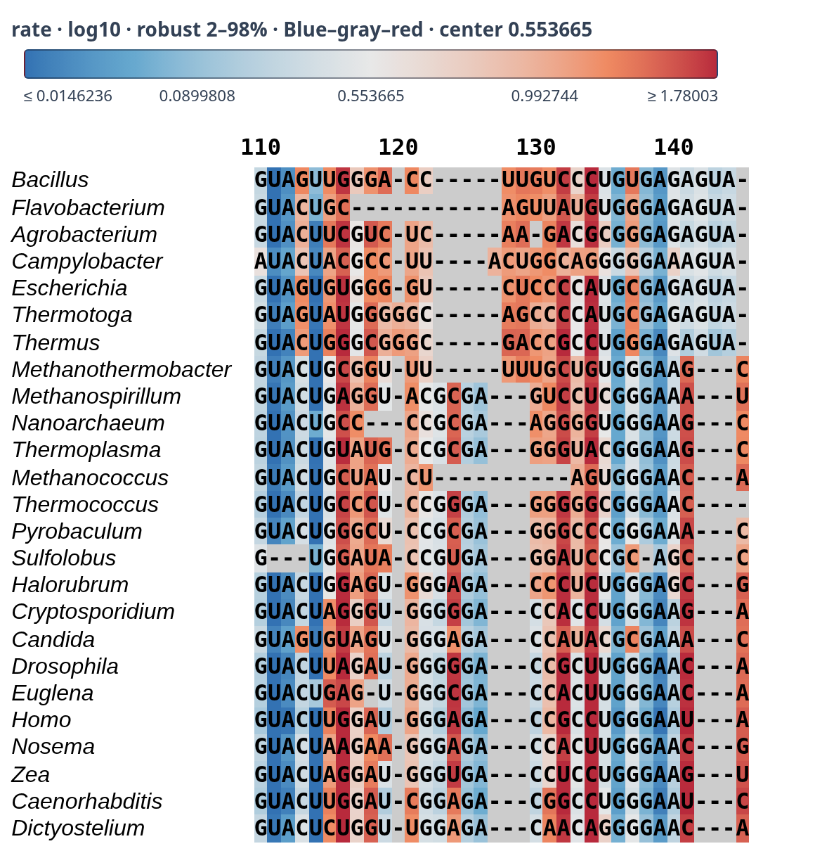
Letters in the same alignment column can have different inferred rates. Compare the colors among sequences around columns 130–140: blue indicates lower posterior mean rates and red higher rates. These estimates average over sampled alignments and are displayed here on the AMA alignment. The colors summarize rate variation under the covarion model; they do not provide a formal test for heterotachy.
To explore this example, open the
interactive
alignment. Select rate, clear Original colors,
and choose Log10, Blue–gray–red, and
Robust (2–98%).
The Log10 scale retains rate values as legend labels. The robust range assigns the lowest
and highest 2% of values to the endpoint colors.
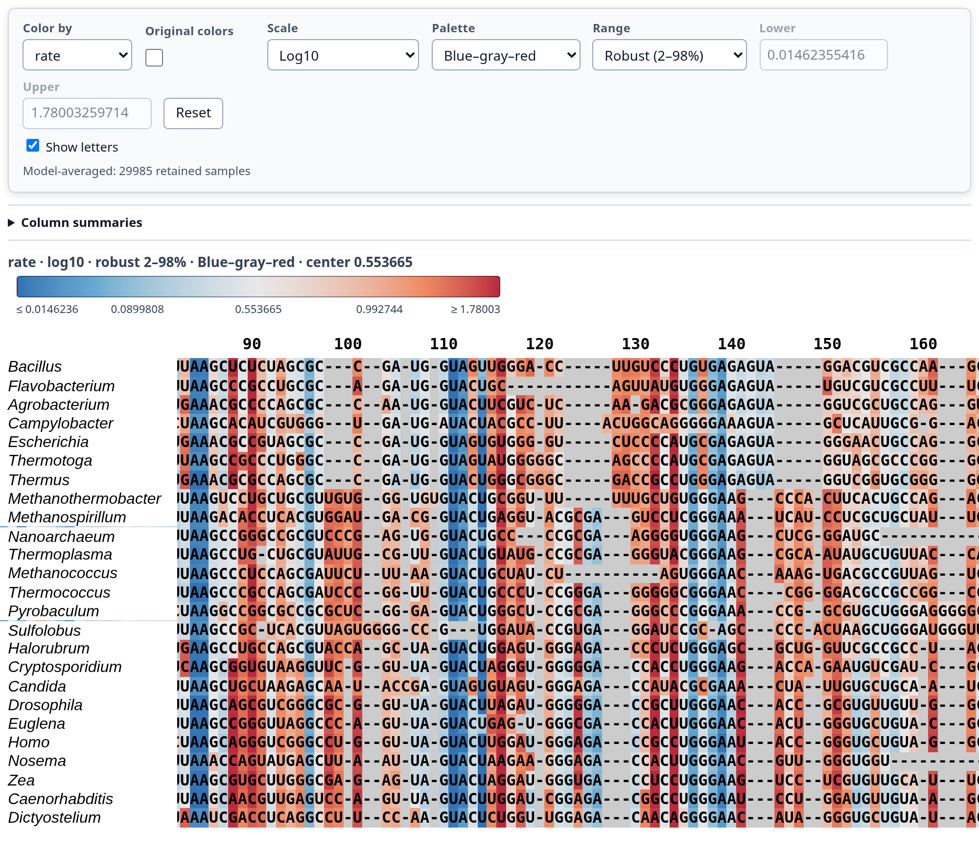
The legend explains the alignment colors. Expand
Column summaries to inspect numerical results.
Open Column summaries to inspect or sort the numerical table,
then select a column number to locate it in the alignment. Summaries start collapsed for
both rates and positive-selection properties. In AU views, Fade by AU
fades colors according to alignment uncertainty; leave it off to compare rates alone.
Clear Show letters to compare background colors without the
sequence letters. You can still point to cells to inspect their estimates.
Supported properties are logged automatically in
C1.P1.site-property-samples.jsonl for partition 1, and similarly for
other partitions. To export a table using an alignment of your choice, use
character-properties:
% character-properties summarize run-1/C1.P1.site-property-samples.jsonl \
  run-2/C1.P1.site-property-samples.jsonl --skip=burnin > properties.json
% character-properties report properties.json alignment.fasta rate --format=tsv > rates.tsv
This table summarizes the per-letter rate estimates within each alignment column.
Sequence names and ungapped sequences must match the analyzed data. Sequence positions
identify letters; column numbers refer only to the alignment used for display. See
character-properties report --help for filtering and reporting options.
10. Positive selection
Codon models distinguish synonymous changes, which preserve the amino acid, from nonsynonymous changes, which alter it. The parameter \(\omega\) (often called dN/dS) multiplies the nonsynonymous rates in a codon model. Values below one reduce these rates; values above one increase them and represent diversifying positive selection. Here positive selection means an excess of amino-acid changes relative to the model's background rates, not evidence that a particular mutation is advantageous.
Use homologous protein-coding sequences in the correct reading frame. Remove terminal
stop codons and check for internal stops or frameshifts. The commands below assume the
standard genetic code. By default, BAli-Phy estimates the alignment along with selection;
add -I none to hold the input alignment fixed.
Alignment uncertainty is included in the character summaries
(Section 9, “Character properties”). An alignment model does not correct sequencing
errors, incorrect gene boundaries, or recombination.
Choose an analysis according to the question you want to answer:
| Question | Analysis |
|---|---|
| What is the overall dN/dS? | Single-ω analysis |
| Is there evidence of positively selected sites? | Site test |
| Does dN/dS differ between branch groups? | Branch test |
| Is there evidence of selection at some sites on specified branches? | Branch-site test |
A branch test detects differences in ω, which need not involve positive selection. After assessing evidence for selection in the gene, you can locate codons with evidence of selection and display their probabilities on an alignment.
10.1. Bayesian tests in BAli-Phy
BAli-Phy uses Bayesian model comparison to assess support for competing hypotheses. Its tests include those hypotheses within a single analysis. During MCMC sampling, the analysis can move between them. A variable called the model indicator records which hypothesis is currently active. Its posterior distribution tells us how much probability the analysis assigns to each hypothesis, given the data and priors.
The site models, BranchModel,
BranchModel_test, and BranchSite
share the default background GTR +> MNM +> MutSelAA.
Their ω values scale nonsynonymous rates relative to that background. A category called
neutral (ω=1) retains amino-acid fitness effects; positive selection refers to excess
nonsynonymous change beyond that background. The mutation and fitness parameters are
shared across categories, branch groups, and competing hypotheses.
Site and branch-site tests compare a hypothesis that allows positive selection with one that does not. Branch tests compare hypotheses about how ω varies among branches; a difference in ω need not involve positive selection. Unlike CODEML's likelihood-ratio tests, these comparisons do not require fitting the competing models separately. Support is summarized using posterior probabilities and Bayes factors.
For parameters and default priors, consult the
M8a_test function reference
or run bali-phy help M8a_test. Other models have corresponding help pages.
The following subsections explain which models to run and where to find their
results in the reports generated by bpy-summarize. Bayes factors
describe how strongly the data shift support toward one hypothesis over another.
See Section 10.7, “Interpreting support for competing hypotheses” for their interpretation and their
relationship to posterior probabilities.
10.2. One ω for the whole sequence
Start with a model that uses one ω for all sites and branches:
% bali-phy coding.fasta -A Codons -S 'GTR +> MNM +> MutSelAA +> dNdS'GTR describes nucleotide mutation.
MNM allows mutations to change one, two, or three nucleotides
within a codon.
MutSelAA estimates amino-acid preferences shared across sites, and
dNdS adds the ω multiplier. Here ω describes nonsynonymous change
beyond the effect of those preferences; it is not a raw ratio of observed changes.
Setting ω to one leaves those preferences intact, rather than removing all selection.
MutSelAA assigns equal fitness to synonymous codons.
To allow separate codon preferences, use MutSel instead:
% bali-phy coding.fasta -A Codons -S 'GTR +> MNM +> MutSel +> dNdS'Both models estimate preferences shared across sites. The examples below use
MutSelAA because MutSel currently mixes
substantially more slowly and thus needs longer runs for reliable estimates.
See Section 10.9, “Codon frequencies and the background model” and
Section 10.11, “Multinucleotide mutations” for the reasons behind these background-model choices.
The default LogNormal(0,1) prior gives equal probability to
ω below and above one. To restrict ω to values below one, use
dNdS(omega=~Uniform(0,1)). Run independent chains, check convergence,
and summarize them as in Section 4.2, “Posterior summaries”. Read the ω estimate and credible
interval in the parameter report. A single ω cannot identify selected sites, and averaging
across the sequence can hide selection affecting only a few sites.
10.3. Different ω values among sites
A site model allows ω to differ among codon sites. Each site belongs to an unknown category with its own ω, which applies on every branch. The analysis estimates the category proportions, any unknown ω values, and each site's probability of belonging to each category.
M1a has two categories: ω below one and ω equal to one. M2a adds a category with ω above one. M7 uses a beta distribution for ω between zero and one, approximated by a finite set of categories. M8a adds a category with ω equal to one; M8 instead adds one with ω above one.
Use M2a_test to compare M1a with M2a, or
M8a_test to compare M8a with M8. In each comparison, the selection
hypothesis includes a category with ω above one; the null hypothesis does not.
Each command allows the chain to move between the two hypotheses:
% bali-phy coding.fasta -A Codons -S M2a_test
% bali-phy coding.fasta -A Codons -S M8a_test
For example, M8a_test expands to:
|w:GTR +> MNM +> MutSelAA +> dNdS(omega=w)| +> M8a_testThe expression |w:...| builds the codon model for a supplied
ω value. The site model supplies these values and their priors, rather than using the
single-ω default prior. To include positive selection throughout the analysis without comparing
hypotheses, replace M2a_test with M2a, or
M8a_test with M8.
See Section 10.7.1, “Reading the summary report” for reading model support in the report. The following section explains how to examine individual codons.
10.4. Locating positively selected codons
After assessing evidence for positive selection in the gene
(Section 10.7, “Interpreting support for competing hypotheses”), examine the site table in the
bpy-summarize positive-selection report. It gives probabilities that
individual codons have ω above one. These estimates account for alignment uncertainty
by following each codon across sampled alignments (Section 9, “Character properties”).
Overall posterior averages over both the selection and
no-selection hypotheses. Posterior with selection is conditional on
the selection hypothesis. For example, a codon with conditional probability 0.95 has
overall probability 0.19 if the selection hypothesis has posterior probability 0.20.
Mean dNdS estimates ω; it is not a selection probability.
To display these probabilities on an alignment, choose posSelection
in the alignment viewer. There, the overall and conditional summaries are labelled
Model-averaged and
Conditional on positiveSelectionInModel, respectively.
When the alignment is uncertain, codons in the same displayed column can occupy different columns in sampled alignments, and therefore have different selection probabilities. The site table represents each column by the codon with the highest conditional probability, or the highest overall probability if conditional estimates are unavailable. Its sequence name and ungapped position identify the observed codon; the displayed letter is not an inferred ancestral or consensus codon.
The table shows up to 20 columns that pass the display threshold.
All rows (TSV) exports every column, regardless of the threshold.
The threshold controls the display; it is not a significance test.
Conditional estimates may be imprecise when few samples were drawn under the selection hypothesis. With no such samples, these estimates are unavailable.
10.5. Different ω values among branches
A branch model assigns branches to numbered categories, each with one ω shared across
all sites. Several branches can share a category. Fix the topology and label branches in a
Newick tree containing all your sequences. Save it as branches.tree.
This four-sequence example is an unrooted tree and labels
the branch separating A and B from C and D:
branches.tree((A,B):[&foreground=1],C,D);The label follows a colon because it belongs to the branch, not the node. This assigns that branch to category 1; unlabelled branches use category 0. Branch lengths are still estimated:
% bali-phy coding.fasta -A Codons --fix topology=branches.tree \
  -S '|w:GTR +> MNM +> MutSelAA +> dNdS(omega=w)| +> BranchModel'
The Branch models report summarizes the category ω values.
A category number identifies a shared parameter, not a particular branch. Different
branch groups can have different ω values while all remain below one.
To test whether the labelled branch needs a separate ω, change its label to
[&foreground={0,1}] and replace BranchModel
with BranchModel_test in the command. In this example, hypothesis 0
uses category 0 everywhere; hypothesis 1 uses category 1 on that branch.
Each entry in the label gives that branch's category under a hypothesis: the first
entry is for hypothesis 0, the second for hypothesis 1, and so on. Thus,
[&foreground={1,0}] reverses the assignments on that branch.
Unlabelled branches use category 0 under every hypothesis.
The report gives the probability of each hypothesis and separate ω summaries using only samples from that hypothesis. These tables omit unused categories. Summaries across all hypotheses include prior draws whenever a category is unused. This tests whether ω differs among branches, not specifically whether it exceeds one. See Section 10.7.1, “Reading the summary report” for reading support for the hypotheses in the report.
10.6. Selection at some sites on designated branches
A branch-site model distinguishes branches of interest, called foreground branches,
from the remaining background branches. Some sites can have ω at or below one on background
branches but ω above one on foreground branches. BranchSite
compares this with a null hypothesis in which those sites have ω equal to one on the
foreground branches. The analysis estimates which sites are affected and the ω shared by
these sites on foreground branches.
Use a fixed topology with [&foreground=1] on foreground branches,
as in the first tree above, not the {0,1} label used for
BranchModel_test. Leave background branches unlabelled:
% bali-phy coding.fasta -A Codons --fix topology=branches.tree \
  -S '|w:GTR +> MNM +> MutSelAA +> dNdS(omega=w)| +> BranchSite'
Read model support as in Section 10.7.1, “Reading the summary report” and the two
posterior views as in Section 10.4, “Locating positively selected codons”. In the alignment
viewer, foreground-posSelection gives selection probabilities and
foreground-dNdS gives ω estimates on foreground branches.
background-posSelection and background-dNdS
describe the same sites on background branches. Fixing the topology does not fix the
alignment. Choose foreground branches from the biological question before examining
selection results. Searching many branch sets and reporting only the strongest result can
exaggerate the evidence.
10.7. Interpreting support for competing hypotheses
Posterior probabilities describe support for the competing hypotheses given the data and priors. Each probability refers to a hypothesis as a whole. In a branch test, the hypotheses describe different ways of assigning ω values to branches.
For a two-hypothesis selection test, a posterior probability of 0.9 for the selection hypothesis means a probability of 0.1 for the no-selection hypothesis. These probabilities describe support for the competing models, rather than selection at a particular codon. See Section 10.4, “Locating positively selected codons” for interpreting individual-codon probabilities.
The odds in favor of one hypothesis over another are the ratio of their probabilities. A Bayes factor measures how the data change those odds: it is the posterior odds divided by the prior odds. For hypotheses A and B:
\[\mathrm{BF}_{A:B} = \frac{\Pr(A\mid D)/\Pr(B\mid D)}{\Pr(A)/\Pr(B)}\]
Here D denotes the data. The site and branch-site tests give their two alternatives equal prior probability by default, so posterior odds equal the Bayes factor. In the example above, posterior probabilities of 0.9 and 0.1 give a Bayes factor of 9 in favor of selection. With unequal prior probabilities, divide the posterior odds by the prior odds even when comparing only two models.
The same formula applies to a pair of alternatives when there are more than two. To compare one alternative with all the others together, sum the others' probabilities in both the posterior and prior odds. Even with equally probable alternatives, the prior odds of one against the rest are not one unless there are only two alternatives.
Model support averages over uncertainty in parameters and, when the alignment is estimated, over alignments. Parameter priors therefore matter as well as the prior probabilities of the models. See Section 10.13, “Comparing with CODEML” for how this differs from likelihood-ratio tests.
10.7.1. Reading the summary report
Open Results/index.html, generated by
bpy-summarize. For site and branch-site tests, find
Support for positive selection in the model under
Positive selection. The Posterior probability
column gives support for the selection hypothesis; Log odds compares
it with the no-selection hypothesis. For the site-level tables below it, see
Section 10.4, “Locating positively selected codons”.
For branch tests, find Hypothesis support under
Branch models. Each row gives a hypothesis's
Posterior probability and Posterior log odds
against all other hypotheses combined. Used categories lists the
ω categories used under that hypothesis. Hypotheses have equal prior probability by
default.
Both tables report posterior log odds, not log Bayes factors. Subtract the corresponding prior log odds to obtain a log Bayes factor, using the comparisons described above.
These tables are especially useful when one hypothesis has very little support. Counting how often each hypothesis was sampled can give a probability estimate of exactly zero or one if the rare hypothesis never appears. For example, with posterior log odds of 50, the less probable hypothesis has probability approximately \(e^{-50}\). Roughly \(e^{50}\) independent samples would be needed merely to expect one occurrence, and more would be needed for a reliable frequency estimate.
The support tables use conditional probabilities calculated at each MCMC sample, rather than relying only on which hypothesis was active. They can therefore retain information about a hypothesis even when the indicator never takes that value. Calculating with logged conditional odds also avoids losing this information when ordinary probabilities round to zero or one. The analysis must still explore the relevant parameter distributions adequately.
Related quantities can also appear under Scalar variables.
When present, their means have the following interpretations:
| Quantity | Meaning of its mean |
|---|---|
posSelection | Fraction of retained samples in which selection is active. This can be exactly zero or one when one hypothesis is rarely sampled. |
PrPosSelection | Estimates posterior selection probability using conditional probabilities, rather than only counting indicator values. |
PrBranchHypothesis[i] | Estimates posterior support for hypothesis i using
conditional probabilities. |
hypothesis | Average of numerical hypothesis labels; not generally a hypothesis probability. |
LogOddsPosSelection,
LogOddsBranchHypothesis[i] | Average conditional log odds, not the posterior log odds shown in the dedicated support tables. |
Use the dedicated support tables to interpret model evidence. Even means of conditional probabilities can round to zero or one; the log-odds summaries retain information that those rounded probabilities cannot show.
10.7.2. Text output and logged quantities
bpy-summarize uses statreport to produce these
summaries. To inspect a text summary directly, you can also run:
% statreport --skip=burnin run-1/C1.log run-2/C1.logstatreport uses the logged conditional odds to estimate posterior
probabilities and log odds. It combines the probabilities of a hypothesis and its
alternatives separately, calculating on the log scale to preserve very small values.
Do not average the logged odds directly: the mean of conditional log odds is not the
log odds of the posterior hypothesis probability. For branch tests, the reported log
odds compare each hypothesis with all other hypotheses combined.
10.8. Model assumptions and false positives
A false positive is an inference of positive selection when it is absent. Evidence for selection depends on which changes the model expects without it. If the background model assigns those changes too little probability, increasing ω can partly compensate for the error. This can improve the fit without correctly explaining the process: ω increases only nonsynonymous rates, rather than correcting the background model.
A better background can strengthen or weaken evidence for selection. The following subsections explain the background choices in the examples, how alignment uncertainty is handled, and how to add synonymous rate variation. These choices improve robustness to particular sources of systematic error; they do not prevent all false positives.
10.9. Codon frequencies and the background model
Goldman–Yang (GY) models weight a change by the frequency of the destination codon. Muse–Gaut (MG) models instead use the frequency of the nucleotide being introduced. For example, for AGA → AGT, a GY model uses the frequency of AGT, whereas an MG model uses the frequency of T. With codon frequencies calculated as products of nucleotide frequencies, the GY rate therefore includes factors for the unchanged A and G as well. These different backgrounds can lead to different conclusions about selection, including false positives or missed selection (Yap et al. 2010).
The mutation–selection models used here separate nucleotide mutation biases from
amino-acid or codon preferences. Rates depend on mutation rates and fitness differences,
rather than directly multiplying by the destination-codon frequency. This separates two
causes of unequal codon usage and motivates using MutSelAA or
MutSel in the examples. It does not remove all assumptions about
the background process.
10.10. Alignment error and uncertainty
Aligning unrelated codons can create apparent amino-acid substitutions and spurious evidence of selection. BAli-Phy jointly estimates alignment and selection, allowing each hypothesis to be evaluated over plausible alignments instead of treating one alignment as certain. In branch-site simulations, this removed the excess false positives caused by alignment error while detecting selection nearly as often as when the true alignment was known (Redelings 2014).
The examples above already sample alignments. Omit -I none
to retain this behavior. Fixing the topology for a branch or branch-site analysis does not
fix the alignment. See Section 9, “Character properties” for interpreting site results
across sampled alignments.
10.11. Multinucleotide mutations
Two or three differences within a codon can arise from one mutation. A model allowing only single-nucleotide mutations must explain them through several events, potentially exaggerating the evidence for positive selection. This effect has been demonstrated for branch-site tests (Venkat et al. 2018).
MNM, already included in the examples, estimates rates of
double and triple mutations as part of the background model. Likelihood evaluation has the
same computational cost as for single-nucleotide mutations; estimating the two additional
parameters may increase the total computation required for inference.
It allows these events within codons, not across codon boundaries. Replace it with
x3 to restrict mutations to single-nucleotide events, as in
Section 10.13, “Comparing with CODEML”.
10.12. Synonymous rate variation
Codons can differ in their baseline substitution rates, affecting synonymous as well as nonsynonymous changes. This is distinct from variation in ω. Ignoring baseline-rate variation can distort evidence for selection (Rubinstein et al. 2011). For comparable nonsynonymous change, a lower inferred baseline rate can strengthen evidence for selection; a higher baseline can weaken it.
Append ASRV.Gamma to add a gamma distribution of rates among
codons:
% bali-phy coding.fasta -A Codons \
  -S '|w:GTR +> MNM +> MutSelAA +> dNdS(omega=w)| +> M8a_test +> ASRV.Gamma'
Each codon now has a rate category as well as an ω category. Its rate multiplier
scales synonymous and nonsynonymous rates together without changing ω, and applies on
every branch. Append ASRV after the completed selection model, outside
|w:...|, as shown. The same distribution of rate multipliers applies
to all ω categories and both hypotheses. This construction works with the other models above.
ASRV.Gamma approximates the gamma distribution with four
categories by default. Alternatively, ASRV.Free estimates category
rates and proportions without requiring a gamma shape. Start with two categories:
% bali-phy coding.fasta -A Codons \
  -S '|w:GTR +> MNM +> MutSelAA +> dNdS(omega=w)| +> M8a_test +> ASRV.Free(n=2)'
The number of categories is fixed by n, not inferred.
If the two estimated rates are clearly separated, try n=3 and check
whether the data distinguish a third rate and mixing remains adequate. The default
of four free-rate categories introduces more parameters. Both ASRV extensions increase
computation by combining rate categories with selection categories, so they are optional
rather than part of the baseline examples.
10.13. Comparing with CODEML
A typical CODEML likelihood-ratio test fits competing models separately and compares their maximized log likelihoods. BAli-Phy's Bayesian tests include the competing models in each analysis: you do not need separate fits or maximized log likelihoods.
| CODEML likelihood-ratio workflow | BAli-Phy Bayesian-test workflow |
|---|---|
| Fit competing models separately | Include competing models in each analysis |
| Compare maximized log likelihoods | Summarize posterior model probabilities and Bayes factors |
| Optimize model parameters | Average over parameter uncertainty under specified priors |
| Condition on a supplied alignment | Fix the alignment or average over alignments |
See Section 10.1, “Bayesian tests in BAli-Phy” for the Bayesian testing workflow, and Section 10.7, “Interpreting support for competing hypotheses” for Bayes factors and their interpretation. Bayes factors are neither likelihood-ratio statistics nor p-values.
The shared-ω versus foreground/background comparison in
Section 10.5, “Different ω values among branches” corresponds to CODEML's M0
(model=0, NSsites=0) versus a labelled branch model
(model=2, NSsites=0). The default BranchSite
compares branch-site model A (model=2, NSsites=2, fix_omega=0)
with its null model fixing ω₂ to one (fix_omega=1, omega=1).
These identify the hypotheses; BAli-Phy compares them using Bayesian model support.
To request the traditional GY94 background explicitly, override
submodel:
% bali-phy coding.fasta -A Codons -I none --fix topology=tree.tree \
  -S 'M8a_test(submodel=(|w:GY94(omega=w)|))'
The model families above correspond to analyses available in PAML's CODEML program,
but the background choices differ. Many earlier analyses used GY94-type models. To compare
with these, use GY94 and match their codon-frequency specification. For example,
GY94(pi=F3x4) uses separate nucleotide frequencies at each codon
position. In a site model, supply ω explicitly:
% bali-phy coding.fasta -A Codons -I none --fix topology=tree.tree \
  -S '|w:GY94(omega=w,pi=F3x4)| +> M8a_test'
The Álvarez-Carretero et al. (2023)
tutorial instead uses FMutSel (CodonFreq=7) with observed codon frequencies
(estFreq=0). The command below uses the same mutation-selection construction,
but infers fitness preferences rather than fixing observed frequencies. It replaces GTR with
HKY85, MNM with x3, and MutSelAA with MutSel:
% bali-phy coding.fasta -A Codons -I none --fix topology=tree.tree \
  -S 'HKY85 +> x3 +> MutSel +> dNdS'
Using MutSelAA instead gives the FMutSel0 fitness structure
(CodonFreq=6); see Section 5.6.2, “Constructing and tweaking codon models” for the full-model
names and their components. For these CODEML models, estFreq=1 estimates
frequencies by maximum likelihood instead of using observed frequencies. This still differs
from Bayesian inference of preferences under priors.
CODEML's hkyREV=0 selects HKY-like mutation rates and
hkyREV=1 selects GTR-like rates. Its codon models restrict instantaneous
changes to a single nucleotide; they do not include the MNM extension. See the
PAML manual
for CODEML settings.
Use the same alignment, topology, genetic code, foreground branches, and retained sites in both programs. Omit ASRV if the CODEML analysis did not include it. Matching the model family does not make the analyses identical.
Specify the Beta category count explicitly with
M8a_test(n=10) (the current default).
The extra category is not included in n.
BAli-Phy uses generally unequal quadrature weights, so matching category counts does not
make the approximations identical; see Section 5.6.5, “Heterogeneous dN/dS and tests for positive selection”.
For the non-clock codon analyses compared here, CODEML reports branch lengths in expected nucleotide substitutions per codon; BAli-Phy uses expected nucleotide substitutions per nucleotide site. Divide CODEML lengths by three to compare units. For partitioned BAli-Phy analyses, use lengths scaled for the codon partition.
A CODEML result with p < 0.05 does not imply a posterior probability of positive selection above 95%. A p-value measures how unusual the test statistic would be under the hypothesis of no positive selection; it is not the probability that this hypothesis is true. A posterior probability measures support for a hypothesis given the data, model, and priors. Thus, CODEML can give a significant result when BAli-Phy reports posterior support below 95%, even with the same likelihood function. These are different criteria for assessing evidence, not equivalent thresholds.
For comparison with CODEML's site probabilities under the selection model, use
Posterior with selection, not Overall posterior
(Section 10.4, “Locating positively selected codons”). Both the BEB result and this conditional summary
assume the selection model, rather than averaging over selection and no-selection models.
For some models, CODEML uses Bayes empirical Bayes (BEB) to account for uncertainty in the parameters describing variation in ω among sites when calculating site probabilities (Yang, Wong, and Nielsen 2005). Other parameters, such as branch lengths, remain fixed at their maximum-likelihood estimates. BAli-Phy averages over uncertainty in all parameters being inferred, for site probabilities and other estimates alike, so no separate BEB correction is needed. Quantities fixed by the user, such as the topology, remain fixed.
11. Ancestral sequence reconstruction
11.1. Ancestral sequences with gaps
BAli-Phy can reconstruct ancestral sequences for all internal nodes. Unlike some programs,
BAli-Phy explicitly infers the presence and absence of characters in ancestral sequences. This
means that if the ancestral sequence has no character for a column, the reconstructed
ancestor will have a gap there. BAli-Phy reconstructs ancestors for fixed-alignment partitions
as well as variable-alignment partitions, but it won't write out fixed alignment samples unless
you add the flag --set write-fixed-alignments=true. Additionally, if you
have an ambiguous character such as N in an observed sequence BAli-Phy
will impute this character.
11.2. Generating a consensus alignment with ancestral sequences
BAli-Phy can reconstruct ancestral sequences for a given tree topology and (leaf sequence) alignment. This is similar to the ancestor-reconstruction that is usually done for fixed-alignment analyses. However, it is not quite the same, because of uncertainty in the tree and the alignment. When computing the probability of an ancestral residue, this summary averages over uncertainty in the topology, the alignment, and the ancestral state itself.
This example uses the original run files and discards iterations 0–999 from each run. Replace 1000 with a burn-in appropriate for your runs. For older PowerShell versions, see Section 3.4.1, “Pipelines and redirected output” before running these pipelines. First, construct the tree topology to annotate:
% trees-consensus --skip=1000 dir-1/C1.trees dir-2/C1.trees | tree-tool - --strip-internal-names --name-all-nodes > c50.treeConstruct the leaf-sequence alignment to annotate using posterior decoding:
% cut-range dir-1/C1.P1.fastas dir-2/C1.P1.fastas --skip=1000 | alignment-chop-internal --tree c50.tree | alignment-max --out P1-max.fastaFinally, reconstruct the ancestral sequences on the given tree and alignment:
% summarize-ancestors P1-max.fasta -A dir-1/C1.P1.fastas -T dir-1/C1.trees -A dir-2/C1.P1.fastas -T dir-2/C1.trees --skip=1000 -n c50.tree > P1.ancestors.fastaThe default --subsample=10 matches one saved alignment to every
tenth tree before applying burn-in. Use --until to set the last retained
iteration and --thin to thin the eligible pairs. Do not remove internal
sequence names or tree labels from the original sample files.
For codon data, pass the same --alphabet option to
alignment-max and summarize-ancestors, for example
--alphabet="Codons(DNA,standard)". Use the genetic code from your analysis.
BAli-Phy uses an alignment estimate (here, P1-max.fasta) as a
template to construct a consensus alignment with ancestral sequences. BAli-Phy doesn't
condition on the alignment columns, because (i) many columns occur only once in a posterior
sample and (ii) conditioning on the column gives too much weight to the template
alignment.
Because the alignment is uncertain, residues in the same column of the template alignment may end up in different columns in an MCMC sample. Therefore, in a given MCMC sample, different leaf residues in the same column may have different ancestors at the same internal node! However, in our ancestral reconstruction, a given column may only display a single ancestral residue.
BAli-Phy addresses this problem by averaging across the different ancestral residues in each column of the template alignment. When identifying the ancestral character for column C from a sampled alignment A, we randomly select a residue in C and use it to select a column from A. This procedure has the nice property that it will yield the traditional ancestral residue prediction if the alignment column is fixed.
11.3. Sampled alignments contain ancestral sequences
Ancestral sequences are written as part of the alignment matrix in each iteration. Ancestral sequences
are given names starting with the letter A. For example, in the
following alignment, the sequences A5, A6, and
A7 are reconstructed ancestors:
>Halobacterium
-T-TAAGGCGGCCATAGCGGTGGGGTTACTCCCGTAC
>Pyrococcus
GG-TACGGCGGTCATAGCGGGGGGGCCACACCCGGTC
>Sulfolobus
GC-CCACCCGGTCACAGTGAGCGGGCAACACCCGGAC
>Homo
GTCTACGGC---CATACCACCCTGAACGCGCCCGATC
>Escherichia
TG-CCTGGCGGCCGTAGCGCGGTGGTCCCACCTGACC
>A5
GG-CAAGGCGGCCATAGCGGGGGGGCCACACCCGGCC
>A6
GT-CAAGGCGGCCATAGCGGGGGGGCTACACCCGGTC
>A7
GT-CAAGGCGGCCATAGCGGGGGGGCTACACCCGGTC
Sampled alignments for the nth partition are in the file.
C1.Pn.fastas.
Ancestral states in these alignments are randomly sampled from their joint posterior and do not represent the most probable ancestral state. The alignment of ancestral sequences is also inferred, so these sequences may contain gaps. The length of ancestral sequences may vary between samples when the length of the ancestral sequence is uncertain.
11.4. Sampled alignments correspond to specific sampled trees
Each sampled alignment matrix corresponds to a tree in the file C1.trees
that is written in the same iteration. This tree specifies the phylogenetic location of each
ancestral sequence by labelling the internal nodes of the tree. For example, the tree below
shows where the internal nodes A5, A6, and A7 are
located on the tree:
(Halobacterium:0.213240,((Escherichia:0.435762,Pyrococcus:0.122678)A5:0.114725,Sulfolobus:0.427210)A6:0.042527,Homo:0.427026)A7;
While the tree is written every iteration, the alignment is only written every 10 iterations
(by default) in order to save disk space. One method for extracting the trees that correspond
to saved alignments is to extract every 10th tree with the program
bpy-subsample:
% bpy-subsample 10 < C1.trees > C1.10.treesLet Command Prompt handle the input and output redirection:
PS> cmd /c "bpy-subsample 10 < C1.trees > C1.10.trees"11.5. Using the sampled alignments instead of a consensus
Instead of constructing consensus ancestral sequences, you can also summarize the sampled alignments and their ancestral sequences directly. This approach involves performing a downstream analysis on each sampled (alignment,tree) pair, yielding the posterior distribution of the downstream analysis. Averaging these results then yields the posterior mean analysis result.
When this approach is feasible, it is more statistically rigorous than analyzing the consensus ancestral sequence alignment. The consensus ancestral sequence alignment does not account for uncertainty in the ancestral sequences, and is not a joint reconstruction. In contrast, analyzing the posterior samples accounts for uncertainty in the ancestral sequences, the alignment, and the tree. Furthermore, it also summarizes joint reconstructions instead of a marginal reconstruction.
11.6. Tree uncertainty in ancestral sequence reconstruction.
In Bayesian phylogenetic analyses, the tree is not fixed. Therefore the internal node corresponding to the ancestral sequence you wish to reconstruct may not exist in every posterior sample. The standard Bayesian approach to tree uncertainty is to reconstruct the ancestor for each node by conditioning on the existence of that node in the tree. This allows the reconstructed ancestor for each node to average over uncertainty about the existence of other nodes.
BAli-Phy additionally allows the researcher to condition on branches, since a branch condition is less restrictive. BAli-Phy does not run a separate MCMC chain with a tree constraint for each node, but instead performs conditioning by selecting samples from a single run that satisfy the condition.
11.6.1. Extracting and naming sequences that satisfy a query
Note that the sequence names (e.g. A6) for internal nodes may change over time. Therefore, you cannot simply extract ancestral sequences with a given name. To extract ancestral sequences for a given node, you need to specify a method of identifying that node on a tree, and a name to give to the sequence at that node. This is called a query.
For example, you might
specify how to identify the ancestor node of Eukaryotes, and the name "Eukaryotes" to use for the
sequence there. You can then use the program extract-ancestors to
extract ancestral sequences from the sampled trees and alignment, and label them with usable names.
Prepare post-1.fastas, post-1.trees, the corresponding
files for run 2, and c50.tree as in Section 11.2, “Generating a consensus alignment with ancestral sequences”:
% extract-ancestors -A post-1.fastas -T post-1.trees -A post-2.fastas -T post-2.trees --subsample=1 -n c50.tree -g c50.tree > P1.ancestors.fastas-n c50.tree and -g c50.tree specify
node-based queries and branch-based queries.
11.6.2. Conditioning on a node: node-based queries
A node exists in a sampled tree if every branch connected to that node exists in the sampled tree. A node-based query asks for the reconstructed ancestral sequence only from samples where every branch connected to that node exists. A node-based query is more stringent than a branch-based query, since it requires multiple branches to exist.
BAli-Phy allows constructing node-based queries by passing in a Newick tree with labelled internal nodes. A node-based query is automatically constructed from each internal node that is labelled.
11.6.3. Conditioning on a branch: branch-based queries
A branch-based query requires only that a single branch exist in a sampled tree. The branch-based query asks for the reconstructed ancestral sequence on one endpoint of that (directed) branch. When the focus is on changes that occur on a particular branch, this makes more sense than a node-based query.
BAli-Phy allows constructing branch-based queries from a file where every line is either a Newick tree or a named group of taxa. For each line that contains a Newick tree, a branch-based query is automatically constructed from each branch where both endpoints are labelled. For a branch from node1 to node2, the query is named "node2<=node1".
Branch-based query files can also contain lines of the form
name = taxon1 taxon2 ... taxonN12. Convergence and Mixing: Is it done yet?
When using Markov chain Monte Carlo (MCMC) programs like MrBayes, BEAST or BAli-Phy, it is hard to determine in advance how many iterations are required to give a good estimate. The number depends on the specific data set that is being examined. As a result, BAli-Phy relies on the user to summarize the output of a running chain periodically in order to determine when enough samples have been obtained. This section describes a number of techniques to diagnose when more samples must be taken.
Some of the better diagnostics for lack of convergence rely on running at least 2 independent copies of the Markov chain (preferably 4-10) from different random starting points to see if the sampled posterior distributions for each chain are the same. Unfortunately, when the distributions all seem to be the same, this doesn't prove that they have all converged to the equilibrium distribution. However, if the distributions are different then you can reject either convergence or good mixing.
12.1. Definition of Convergence
Convergence refers to the tendency of a Markov chain to "forget" its starting value and become typical of its equilibrium distribution. Note that convergence is a property of the Markov chain itself, not of individual runs of the Markov chain. Ideally a number of individual runs should be examined in order to determine how many initial iterations to discard as "burnin".
12.2. Definition of Mixing
In MCMC, each sample is not fully independent of previous samples. In fact, even after a Markov chain has converged, it can get "stuck" in one part of the parameter space for a long time, before jumping to an equally important part. When this happens, each new sample contributes very little new information, and we need to obtain many more samples to get good precision on our parameter estimates. In such a case, we say that the chain isn't "mixing" well.
12.3. Diagnostics: Variation in split frequencies across runs (ASDSF/MSDSF)
12.3.1. ASDSF and MSDSF
To calculate the ASDSF and MSDSF run:
% trees-bootstrap dir-1/C1.trees dir-2/C1.trees ... dir-n/C1.trees > partitions.bsHowever, it is also useful to consider the maximum of the SDSF values (MSDSF). This is the largest standard deviation of split frequencies across runs.
12.3.2. Split-frequency comparison plot
To generate the split-frequency comparison plot, you must have R installed. Locate the script compare-runs.R. Then run:
% trees-bootstrap dir-1/C1.trees dir-2/C1.trees ... dir-n/C1.trees --LOD-table=LOD-table > partitions.bs
% R --slave --vanilla --args LOD-table compare-SF.pdf < compare-runs.R12.4. Diagnostics: Potential Scale Reduction Factors (PSRF)
Potential Scale Reduction Factors check that different runs have similar posterior distributions. Only numerical variables may have a PSRF. To calculate the PSRF for each numerical parameter, you may run:
% statreport dir-1/C1.log dir-2/C1.log ... dir-n/C1.log > Report We compare the PSRF based on the length of 80% credible intervals (Brooks and Gelman 1998) and report the result as PSRF-80%CI. For integer-valued parameters, we add 1 to both the pooled and within-run interval widths before taking their ratio, since an integer interval from \(a\) to \(b\) contains \(b-a+1\) values.
We also report a new PSRF that is more sensitive for integer distributions. For each individual distribution, we find the 80% credible interval. We divide the probability of that interval (which may be more than 80%) by the probability of the same interval under the pooled distribution. The average of this measure over all distributions gives us a PSRF that we report as PSRF-RCF.
This convergence diagnostic gives a criterion for detecting when a parameter value has stabilized at different values in several independent runs, indicating a lack of convergence. This situation might occur if different runs of the Markov chain were trapped in different modes and failed to adequately mix between modes.
12.5. Diagnostics: Effective sample sizes (ESS)
12.5.1. ESS for numerical values
To calculate the ESS values for numerical parameters, run:
% statreport dir-1/C1.log dir-2/C1.log ... dir-n/C1.log > Report Tracer also computes ESS values and displays the numerical traces interactively; see Section 2.9, “Optional programs for inspecting results”.
12.5.2. ESS for split frequencies
As described in Gaya et al. (2011), we can also compute ESS values for splits on the tree:
% trees-bootstrap dir-1/C1.trees dir-2/C1.trees ... dir-n/C1.trees > partitions.bs12.6. Diagnostics: Stabilization
12.6.1. Stabilization of numerical values
To obtain estimates of the stabilization time for each numerical parameter, you may run:
% statreport C1.log > Report 12.6.2. Stabilization of tree topologies and tree distances
In addition to examining convergence diagnostics for continuous parameters, it is important to examine convergence diagnostics for the topology as well (Beiko et al., 2006).
It is also possible to assess stabilization of tree topologies using tools distributed with bali-phy by using commands like the following. Here, subsampling and burnin do not apply to the equilibrium tree files. Also, note that you need to manually construct the equilibrium samples, which we recommend should contain at least 500 trees; you might do this by subsampling using the BAli-Phy tool bpy-subsample.
To report the average distances within and between two tree samples:
% trees-distances --skip=burnin --subsample=factor compare dir-1/C1.trees dir-2/C1.treesTo compute the distance from each tree in C1.trees to all trees equilibrium.trees, as a time series:
% trees-distances --skip=burnin --subsample=factor convergenceC1.treesequilibrium.treesTo assess when the above time series stabilizes:
The stabilization criterion is the same one described above for numerical values.% trees-distances --skip=burnin --subsample=factor convergedC1.treesequilibrium.trees
Note that the running time is the product of the number of trees in the two files. Therefore, comparing two complete tree samples without sub-sampling will take too long.
13. Alignment utilities: brief overview
This section gives a brief overview showing some of the things that can be done with the included alignment utilities. It is intended to be helpful, but not exhaustive. To see the full set of options for each tool, give the argument "--help" on the command line.
13.1. alignment-info
Show basic information about the alignment:
% alignment-info file.fasta
% alignment-info file.fasta file.tree13.2. alignment-cat
To select columns from an alignment:
% alignment-cat -c1-10,50-100,600- file.fasta > result.fasta
% alignment-cat -c5-250/3 file.fasta > first_codon_position.fasta
% alignment-cat -c6-250/3 file.fasta > second_codon_position.fasta
To concatenate two or more alignments:
% alignment-cat file1.fasta file2.fasta > all.fasta13.3. alignment-thin
Remove columns without a minimum number of letters:
% alignment-thin --min-letters=5 file.fasta > file-thinned.fastaRemove sequences by name:
% alignment-thin --remove=seq1,seq2 file.fasta > file2.fastaRemove short sequences:
% alignment-thin --longer-than=250 file.fasta > file-long.fastaRemove sequences with fewer than 5 directional mismatches from the closest other sequence:
% alignment-thin --cutoff=5 file.fasta > more-than-5-differences.fastaLike --cutoff, but stop when we have the right number of sequences:
% alignment-thin --down-to=30 file.fasta > file-30taxa.fastaProtect some sequences from being removed:
% alignment-thin --down-to=30 file.fasta --protect=seq1,seq2 > file-30taxa.fastaRemove sequences that are missing conserved columns:
% alignment-thin --remove-gappy=10 file.fasta > file2.fasta13.4. alignment-draw
Draw an alignment to HTML, optionally coloring residues by AU.
%  alignment-draw file.fasta --show-ruler --color-scheme=DNA+contrast > file.html
% alignment-draw file.fasta --show-ruler --AU=file-AU.prob --color-scheme=DNA+contrast+fade+fade+fade+fade > file-AU.html13.5. alignment-find
Find the last (or first) FastA alignment in a file.
% alignment-find --first < file.fastas > first.fasta
% alignment-find < file.fastas > last.fasta13.6. alignment-chop-internal
Remove ancestral sequences from each alignment, keeping sequences whose names occur as leaves in the specified tree.
% alignment-chop-internal --tree tree < file.fastas > file-chopped.fastas14. Tree utilities: brief overview
This section gives a brief overview showing some of the things that can be done with the included tree utilities. It is intended to be helpful, but not exhaustive. To see the full set of options for each tool, give the argument "--help" on the command line.
14.1. trees-consensus
This program summarizes the tree sample contained in file. It reports the MAP topology, the supported taxa partitions (including partial partitions), and the majority consensus topology.
14.2. trees-bootstrap
Usage: trees-bootstrap file1 [file2 ... ] --predicates predicate-file [OPTIONS]
This program summarizes the tree samples contained in file1, file2, etc. It gives the support of each tree sample for each predicate in predicate-file, and reports a confidence interval based on the block bootstrap.
Each predicate is the intersection of a set of partitions, and is specified as a list of partitions or (multifurcating) trees, one per line. Predicates are separated by blank lines.
14.3. trees-to-SRQ
Usage: trees-to-SRQ predicate-file [OPTIONS] trees-file
This program summarizes the tree samples contained in trees-file. It uses them to produce an SRQ plot for each predicate in predicate-file. Plots are produced in gnuplot format, with one point per line and with plots separated by a blank line.
If --mode sum is specified, then a "sum"
plot is produced instead of an SRQ plot. In this plot, the slope of
the curve corresponds to the posterior probability of the event. If the
--invert option is used then the slope of the
curve correspond to the probability of the inverse event. This is
recommended if the probability of the event is near 1.0, because the
sum plot does not distinguish variation in probabilities near 1.0 well.
15. Compiling BAli-Phy
Compiling BAli-Phy is intended to be a relatively painless process. However, most people will want to use the pre-compiled binaries as described in the standard installation instructions at Section 2, “Installation” instead of compiling BAli-Phy themselves. You might want to compile BAli-Phy yourself if you want to
- run BAli-Phy on a non-Intel CPU (such as ARM64 or Alpha).
- run BAli-Phy on a computing cluster.
- test an unreleased version of bali-phy.
- change the optimization options used to compile BAli-Phy in the pre-compiled binaries.
- compile with debugging options to find the cause of a bug, and maybe fix it.
- modify the source code and submit a patch with new functionality.
15.1. Setup
In order to compile BAli-Phy, you need
Use the GNU C++ Compiler (GCC) version 13 or higher, or the Clang compiler version 18 or higher. GCC 13 and Clang 18 are the oldest versions of these compilers tested in CI. The Cairo graphics library is optional, but if it is missing, thedraw-tree tool that
is used to draw consensus trees won't be built. See also Section 2.9, “Optional programs for inspecting results”.
15.1.1. Linux
On Debian and Ubuntu, you can type:
% sudo apt-get install g++ git libcairo2-dev pandoc libboost-all-dev libcli11-dev% sudo apt-get install meson
% meson --version
1.6.0
On computing clusters, you might want to use miniconda to install the build tools.
% conda create -n devel -c conda-forge --strict-channel-priority
% conda activate devel
% conda install meson gxx boost-cpp cmake pkg-config cairo
% export BOOST_ROOT=$CONDA_PREFIX
Otherwise you can install meson through pip3:
% sudo apt-get install python3 python3-pip python3-venv ninja-build
% python3 -m venv meson
% source meson/bin/activate
% pip3 install meson
15.1.2. Mac
On macOS, the simplest way to get a compiler is to install Xcode version 16 (or newer) command line tools, which come with Clang.
% xcode-select --install% brew install git meson cairo pandoc15.1.3. Compile for native Windows using MSYS2
This section is for developers compiling BAli-Phy from source. Users of the native binary package do not need MSYS2. The MSYS2 project provides GCC/MinGW-w64 in its UCRT64 environment to create native Windows executables.
After installing MSYS2, open the MSYS2 UCRT64 shell and perform a full system update:
% pacman -SyuIf the update asks you to close the terminal, reopen the
MSYS2 UCRT64 shell and run pacman -Syu
again. Then install the compiler, build tools, and libraries used by BAli-Phy:
% pacman -S --needed \
  git \
  mingw-w64-ucrt-x86_64-boost \
  mingw-w64-ucrt-x86_64-cairo \
  mingw-w64-ucrt-x86_64-cereal \
  mingw-w64-ucrt-x86_64-eigen3 \
  mingw-w64-ucrt-x86_64-fmt \
  mingw-w64-ucrt-x86_64-gcc \
  mingw-w64-ucrt-x86_64-meson \
  mingw-w64-ucrt-x86_64-range-v3 \
  mingw-w64-ucrt-x86_64-zstd
pacman installs the Python, Ninja, and pkg-config dependencies of
the packaged UCRT64 version of Meson automatically. Cairo is included so that the
draw-tree program is built. The UCRT64 shell refers to drives as
/c/ instead of C:/.
15.2. Clone, Configure, Compile
First check out the code using git:
% git clone https://github.com/bredelings/BAli-Phy.git
% cd BAli-Phy
Then run meson to configure the build process:
% meson setup build --prefix="$HOME/Applications/bali-phy-4.3/" --buildtype=releaseFinally, build and install the software:
% ninja -C build test
% ninja -C build install
bali-phy and its associated tools should then be located in ~/Applications/bali-phy-4.3/bin/. To install to another directory dir, specify --prefix=dir to meson.
15.3. Options: compiler and linker flags
You can select the C++ compiler by setting the CXX variable. A useful example of this is to use g++-14 on systems where g++ invokes a compiler that is too old:
% CXX=g++-14 meson setup build --prefix="$HOME/Applications/bali-phy-4.3" --buildtype=release% CXXFLAGS="-mtune=native -march=native" meson setup build --prefix="$HOME/Applications/bali-phy-4.3"% CPPFLAGS="-I/usr/local/include" LDFLAGS="-L/usr/local/lib" meson setup build --prefix="$HOME/Applications/bali-phy-4.3" --buildtype=release16. Frequently Asked Questions (FAQ)
16.1. Input files
- 1. Does BAli-Phy accept the wildcard characters "N" or "X"? How does it treat them?
- 2. Does BAli-Phy accept "?" characters?
- 3. Does BAli-Phy accept the characters "R" and "Y", etc.?
Does BAli-Phy accept the wildcard characters "N" or "X"? How does it treat them?
Yes, BAli-Phy accepts the wildcard characters "N" (for DNA) and "X" (for proteins). These characters indicate that some letter is present (as opposed to a gap), but that you don't know which letter it is.
Does BAli-Phy accept "?" characters?
No. "?" characters are often used to indicate either letter presence (e.g. "N", "X") or absence (e.g. "-"). BAli-phy will insist that you replace each "?" with either "N"/"X" or "-" to indicate which one you mean.
(Most programs ignore indels and consider only substitutions, and in that case "N" and "-" have the same effect on the likelihood or parsimony score. However, since BAli-Phy takes indels into account, these two alternatives are quite different.)
Does BAli-Phy accept the characters "R" and "Y", etc.?
Yes. BAli-Phy accepts the characters Y, R, W, S, K, M, B, D, H, and V for DNA, RNA, and Codon alphabets. BAli-Phy also accepts the characters B, Z, and J for amino acids. These characters indicate partial knowledge about a letter. For example, R indicates that a nucleotide is present, and is a puRine (A or G). J indicates that an amino acid is present and is either I or L.
(Note that sequences sometimes contain such ambiguity codes because the DNA that was sequenced contains both values. This might occur when sequencing a heterozygote or when sequencing pooled DNA from several individuals. However, the model in BAli-Phy (and other phylogeny inference programs) is that only one letter is correct, but we do not know which one it is. This is probably not problematic when dealing with pooled sequences, but should be considered.)
16.2. Running bali-phy.
- 1. Can I fix the alignment and ignore indel information, like MrBayes, BEAST, PhyloBayes and other MCMC programs?
- 2. Can I fix the tree topology, while allowing the alignment to vary?
- 3. Can I fix the tree topology and absolute branch lengths in all data partitions, while allowing the alignment to vary?
- 4. Can I fix the tree topology and relative branch lengths, while allowing the alignment to vary?
Can I fix the alignment and ignore indel information, like MrBayes, BEAST, PhyloBayes and other MCMC programs?
Yes. Add -Inone or -I none on the command line.
Can I fix the tree topology, while allowing the alignment to vary?
Yes. Add --fix topology=treefile on the command line.
Can I fix the tree topology and absolute branch lengths in all data partitions, while allowing the alignment to vary?
Yes. Add --fix tree=treefile on the command line.
Can I fix the tree topology and relative branch lengths, while allowing the alignment to vary?
Yes. Add --fix tree=treefile '--scale=~Gamma(0.5,2)' on the command line.
16.3. Run-time error messages
I tried to use -S LG+>ASRV.Gamma(6) and I got an error message "bali-phy: No match." What gives?
You are probably using the C-shell as your command line shell. It is trying to interpret LG+>ASRV.Gamma(6) as an array before running the command, and it is not succeeding. Therefore, it doesn't even run bali-phy.
To avoid this, put quotes around the substitution model, like this: -S 'LG +> ASRV.Gamma(6)'. This will keep the C-shell from interfering with your command.
See Section 3.4, “Shell differences” for quoting in other shells.
16.4. Stopping bali-phy.
- 1. Why is bali-phy still running? How long will it take?
- 2. How do I stop a bali-phy run on my personal computer?
- 3. How do I stop a bali-phy run on a computing cluster?
- 4. So, how can I know when to stop it?
- 5. How can I tell when the chain has converged?
- 6. How can I check how many iterations the chain has finished?
Why is bali-phy still
running? How long will it take?
It runs until you stop it or it reaches its maximum number of iterations. The default maximum is 200,000 iterations; use --iterations to set a different limit.
The longer answer is that it is hard to predict how long MCMC will take to converge, since it depends on each data set in complex ways. Automatic rules for determining when to stop an MCMC chain can be difficult to get right. BAli-Phy does not contain an automatic stopping rule yet, so it relies on the user to run convergence diagnostics and determine when to stop the run.
How do I stop a bali-phy
run on my personal computer?
Simply kill the process -- there is no special
command to stop bali-phy. If you are
running it on your personal workstation, then you can use
the command kill. To do that, you need
to find the PID (process ID) of the running program. You
can find this by examining the beginning of the file
C1.run.json. For
example:
% less 5d-1/C1.run.jsonC1.run.json — excerpt ...
"partitions": [
{
"alphabet": "DNA",
"filename": "5d-muscle.fasta",
"imodel": 0,
"range": "",
"scale": 0,
"smodel": 0
}
],
"pid": 549319,
"program": {
"arch": "linux x86_64",
"build-date": "Mar 2 2024 11:27:23",
"compiler": "gcc 13.2.0 x86_64",
"name": "bali-phy",
"revision": "[HEAD -> master, origin/master, origin/HEAD commit d394a4fb6] (Mar 02 2024 11:11:25)",
"version": "4.0-beta9-preview"
},
...
Here the PID is 549319. Therefore you can type:
% kill 549319On some operating systems you can also use the command below. It will
terminate all of your bali-phy runs
on that computer:
% killall bali-phyHow do I stop a bali-phy
run on a computing cluster?
Simply terminate the submitted job. The specific command to terminate a job will depend on the queue manager that is installed on your cluster. Examine the documentation for your cluster, or ask your cluster support staff how to delete running jobs on your cluster.
As an example, if the SLURM software is used
to submit jobs, then the command squeue
should list your jobs and their job ID numbers (which is
different than the process ID number). You can then use
the command scancel to delete jobs by ID
number. The SLURM documentation describes how to use these
commands.
So, how can I know when to stop it?
You can stop when it has both converged and also run for long enough to give you >1000 effectively independent samples.
How can I tell when the chain has converged?
How can I check how many iterations the chain has finished?
Run wc -l C1.log inside the output
directory, and subtract 2.
16.5. Running bpy-summarize.
- 1. Why does bpy-summarize say "Program 'draw-tree' not found. Tree pictures will not be generated"?
- 2. Why does bpy-summarize say "Program 'R' not found. Some report plots will not be generated"?
- 3. Why is bpy-summarize stopping early, or failing to generate some files?
Why does bpy-summarize say "Program 'draw-tree' not
found. Tree pictures will not be generated"?
The program draw-tree is built only when the Cairo graphics
library is available, so some installations omit it. This is not a fatal error
message; it just means that a picture of the tree will not be generated automatically.
You can still open the tree with TreeViewer or another
program listed in Section 2.9, “Optional programs for inspecting results”.
Why does bpy-summarize say "Program 'R' not found. Some report plots will not be generated"?
R is not installed or is not on your command search path. The report will omit split-support plots, SRQ plots, between-run comparisons, and tree-distance plots. Numerical summaries are still produced.
Why is bpy-summarize stopping early, or failing to generate some files?
Look in the file Results/commands.log. This should contain the specific tool commands that were run, along with error message from these commands. Identify the first tool command that fails, and read the error message.
16.6. Interpreting the results.
How do I compute the clade support?
By default, BAli-Phy uses unrooted trees and reports bi-partition support. A bi-partition divides the taxa into two groups without specifying which contains the root. BAli-Phy also supports rooted tree models; see Section 5.1, “Non-reversible models and rooted trees”.
How do I compute the split/bi-partition support?
After you summarize the output (Section 4.2, “Posterior summaries”), the partition support is indicated in
Results/consensus and in Results/c50.PP.tree.
16.7. How do I...
How do I concatenate alignments?
% alignment-cat filename1.fasta filename2.fasta > result.fastaFor older PowerShell versions, see Section 3.4.1, “Pipelines and redirected output”. The alignments must have the same sequence names, but the names need not be in the same order.
How do I select columns from an alignment?
You can select columns for analysis by specifying a range:
% bali-phy sequences.fasta:1-200,401-600 sequences.fasta:201-400alignment-cat:
% alignment-cat -c1-10,50-100,600- filename.fasta > result.fasta16.8. Installation
Why does an older Bioconda build fail to parse models on Apple Silicon?
Bioconda builds before BAli-Phy 4.2 have a model-parsing bug on Apple Silicon. Install BAli-Phy 4.2 or newer.